4 Introduction to Generalized Linear Models
Author: Grace Tompkins
Last Updated: August 5, 2022
4.1 Introduction
Although linear models have the potential to answer many research questions, we may be interested in finding the association between an outcome and a set of covariates where the outcome is not necessarily continuous or normally distributed. For example, a researcher may be interested in the relationship between the number of cavities and oral hygiene habits in adolescent patients, or perhaps a researcher is interested in identifying covariates that are related to food insecurity in rural populations. In these settings where we do not have a normally distributed outcome, linear regression model assumptions do not hold, and we cannot use them to analyze such data. Generalized linear models (GLMs) are an extension of linear regression models that allow us to use a variety of distributions for the outcome. In fact, linear regression is a special case of a GLM.
In this section, we will introduce the generalized linear model framework with an emphasis for model fitting in R.
4.2 List of R Packages
In this section, we will be using the packages catdata, MASS, AER, performance, faraway , and car. We can load these packages in R after installing them by the following:
4.3 Generalized Linear Model Framework
The generalized linear model is comprised of three components:
The Random Component: The distribution of the independently and identically distributed (i.i.d.) response variables are assumed to come from a parametric distribution that is a member of the exponential family. These include (but are not limited to) the binomial, Poisson, normal, exponential, and gamma distributions,
The Systematic Component: The linear combination of explanatory variables and regression parameters, and
The Link Function: The function that relates the mean of the distribution of \(Y_i\) to the linear predictor through
\[ g(\mu_i) = \beta_0 + \beta_1x_{i1} + \beta_2x_{i2} + ...+ \beta_px_{ip} \] where \(\mu_i = E[Y_i]\) is the mean of outcome and \(x_{i1}, ..., x_{ip}\) are the \(p\) covariates for individual/subject \(i\). We note that there is no error term on this model, unlike in the usual linear regression model. This is because we are modelling the mean of the outcome and thus a random error term is not needed.
4.3.1 Assumptions
We need to satisfy a number of assumptions to use the GLM framework:
- The outcome \(Y_i\) is independent between subjects and comes from a distribution that belongs to the exponential family,
- There is a linear relationship between a transformation of the mean and the predictors through the link function, and
- The errors are uncorrelated with constant variance, but not necessarily normally distributed.
We also assume that there is no multicollinearity among explanatory variables.
Multicollinearity (sometimes referred to as collinearity) occurs when two or more explanatory variables are highly correlated, such that they do not provide unique or independent information in the regression model. If the degree of correlation is high enough between variables, it can cause problems when fitting and interpreting the model. One way to detect multicollinearity is to calculate the variation inflation factor (VIF) for each covariate in a model. The general guideline is that a VIF larger than 10 indicates that the model has problems estimating the coefficients possibly due to multicollinearity. We will show in Section 4.6 how to use R functions to calculate the VIF after model building.
We note that our methodology will be particularly sensitive to these assumptions when sample sizes are small. When collecting data, we also want to ensure that the sample is representative of the population of interest to answer the research question(s).
4.3.2 Link Functions
Recall that we are modelling the mean of the outcome through a link function as in \[ g(\mu_i) = \beta_0 + \beta_1x_{i1} + \beta_2x_{i2} + ...+ \beta_px_{ip}. \] The link function will essentially transform a non-linear outcome to a linear outcome allowing us to fit a generalized linear model. For each distribution in the exponential family, there is a canonical link which is recommended to use as simplifies the process of finding maximum likelihood estimates in our model by ensuring that the mean of our outcome is mapped to \((-\infty, \infty)\) so we do not need to worry about constraints when optimizing. It also ensures \(\boldsymbol{x}^T\boldsymbol{y}\) is a sufficient statistic for \(\boldsymbol{\beta}\).
The following is a table containing commonly used distributions, their canonical links, and the corresponding name used in R:
| Distribution of \(Y\) | Canonical Link | Family parameter in R glm function |
|---|---|---|
| Normal (used for symmetric continuous data) | Identity: \(g(\mu) = \mu\) | family = gaussian(link = "identity") |
| Binomial (Binary data is a special case where n = 1) | Logistic: \(g(\mu) = \log\left(\frac{\mu}{n-\mu}\right)\) | family = binomial(link = "logit") |
| Poisson (used for discrete count data) | Log: \(g(\mu) = \log(\mu)\) | family = poisson(link = "log") |
| Gamma (used for continuous, positive, skewed or heteroskedastic data) | Reciprocal: \(g(\mu) = \frac{1}{\mu}\) | family = Gamma(link = "inverse") |
Each link function will dictate how we interpret the model parameters. For example, using a logistic link for binomial outcome data (also known as logistic regression), we interpret our parameters \(\beta\) as log odds ratios. More details on this can be found in the dedicated logistic regression module in Section 4.6. When using a log link on Poisson data, our model parameters estimate log relative rates, which we will detail in Section 4.8.
We note that sometimes we will use link functions other than the canonical link. For example, it is common for researchers evaluating dose-response relationships for binary outcomes to use the probit link instead of the canonical logistic link. The probit link is the inverse of the standard normal cumulative distribution function. We will also provide a detailed example for this in Section 4.7.2.
To fit a GLM in R, we use the glm() function. In this function, we can specify:
formula: a description of the model to be fit, similar to that in a regular linear model. For example, to fit a glm with outcomeyand covariatesx1andx2, we would writey ~ x1 + x2.family: a description of the error distribution and link function. That is, we specify the type of GLM to fit using the calls in the third column of the above table.data: the name of the data frameweights: (optional) a vector of column of weights.
We will show concrete examples of how to fit different types of GLMs in the following sections.
4.4 Notes on Model Selection
When fitting GLMs, it is important to perform model selection procedures and assess the model fit before interpreting the results. We aim to find a parsimonious model that addresses our research questions. That is, we aim to find the simplest model that explains the relationship between the outcome and covariate(s) of interest.
One of the most common ways to compare models against each other is through the likelihood ratio test (LRT). For the likelihood ratio test, we can compare nested models. That is, we can compare a full model to a nested model that contains a subset of variables that appear in the full model (and no other variables or transformations). Likelihood ratio tests tend to be the preferred method for building logistic regression models where we want to draw claims and perform hypothesis tests.
We typically start model selection with a full main-effects only model and look at removing the least significant covariates in the full model. We can see if these covariates can be removed in the model by testing the full model against one that does not contain those two covariates by a LRT. The LRT compares the residual deviance from both models we are comparing, with degrees of freedom (df) equal to the difference in the number of covariates between the two models. We are specifically testing the null hypothesis \(H_0\): the simpler model is adequate compared to the more complex model. That is, if the \(p\)-value from the test is small, we reject the null and conclude that the simpler model is not adequate, and we should use the fuller model. We can perform an LRT in R by using the anova() function with test = "LRT" in the function call.
For nested or non-nested models, we can also perform model selection by either Akaike information criterion (AIC) or Bayesian information criterion (BIC) where a smaller value represents a better fit. Although both AIC and BIC are similar, research has shown that each are appropriate for different tasks, as discussed here. For the problems discusses in the following sections, AIC and BIC are comparable and either are appropriate for use.
In the following sections, we will outline examples of fitting, assessing, and interpreting various of generalized linear models for commonly used distributions.
4.5 Normally Distributed Outcomes
A generalized linear model with a normally distributed outcome using the canonical link (identity) is the same as a linear regression model.
4.5.1 Example
We will be demonstrating the use of a glm on normally distributed data using the rent data set from the catdata package in R. This data set contains information on 2053 units’ rent (in euros), rent per squared meter (in euros), number of rooms, and other covariates for renal units in Munich in 2003. A full list and description of the variables can be found using by typing ?rent in the R console and reading through the documentation. We read in this data set with the following code, and look at the first 6 observations by;
##     rent rentm size rooms year area good best warm central tiles
## 1 741.39 10.90   68     2 1918    2    1    0    0       0     0
## 2 715.82 11.01   65     2 1995    2    1    0    0       0     0
## 3 528.25  8.38   63     3 1918    2    1    0    0       0     0
## 4 553.99  8.52   65     3 1983   16    0    0    0       0     0
## 5 698.21  6.98  100     4 1995   16    1    0    0       0     0
## 6 935.65 11.55   81     4 1980   16    0    0    0       0     0
##   bathextra kitchen
## 1         0       0
## 2         0       0
## 3         0       0
## 4         1       0
## 5         1       1
## 6         0       0
We wish to see what main factors are related to rental prices, and use this model to predict the rental prices of units not included in the sample.
First, we need to assess the distribution of the outcome. We are going to use rentm, which is the clear rent per square meter in euros, as the outcome of interest. To assess the normality of the outcome, we can plot a histogram of the distribution and create a quantile-quantile (Q-Q) plot. To do so in R, we perform the following commands:
# plot two plots side by side
par(mfrow = c(1,2))

#plot the histogram
hist(rent$rentm, main = "Histogram of Rent per \nSquared Meter",
     xlab = "Rent per Squared Meter")

#plot the qq plot, with reference line
qqnorm(rent$rentm)
qqline(rent$rentm)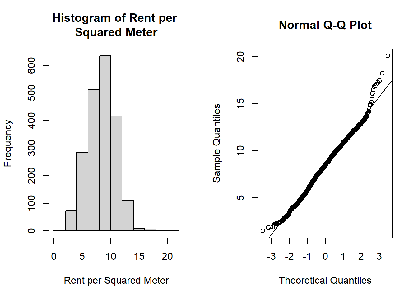
Figure 4.1: Plots Used for Assessing Normality
From the histogram of rentm in Figure 4.1, we see that we have a fairly symmetric distribution. In the Q-Q plot, most points lie on the line, indicating that we have evidence to suggest the normality assumption is satisfied. That is, the normal distribution seems to be an appropriate distribution to assume for our outcome \(Y\) in our GLM.
Let’s fit a generalized linear model to this data set using the glm() function in R, recalling that some covariates are categorical and need to be assigned as a factor() while fitting the model:
# fit a full model
rentm_fit1 <- glm(rentm ~ size + factor(rooms) + year + factor(area) +
                    factor(good) + factor(best) + factor(warm) +
                    factor(central) + factor(tiles) + factor(bathextra) +
                    factor(kitchen), data = rent, family = gaussian(link = "identity"))

# see summary of model
summary(rentm_fit1)
##
## Call:
## glm(formula = rentm ~ size + factor(rooms) + year + factor(area) +
## factor(good) + factor(best) + factor(warm) + factor(central) +
## factor(tiles) + factor(bathextra) + factor(kitchen), family = gaussian(link = "identity"),
## data = rent)
##
## Coefficients:
## Estimate Std. Error t value Pr(>|t|)
## (Intercept) -29.056738 4.353750 -6.674 3.21e-11 ***
## size -0.012989 0.003553 -3.656 0.000262 ***
## factor(rooms)2 -0.962336 0.168848 -5.699 1.38e-08 ***
## factor(rooms)3 -1.222089 0.211164 -5.787 8.27e-09 ***
## factor(rooms)4 -1.464680 0.286182 -5.118 3.38e-07 ***
## factor(rooms)5 -1.262989 0.445118 -2.837 0.004593 **
## factor(rooms)6 -1.348122 0.681699 -1.978 0.048111 *
## year 0.020691 0.002210 9.363 < 2e-16 ***
## factor(area)2 -0.579401 0.355480 -1.630 0.103277
## factor(area)3 -0.649166 0.366119 -1.773 0.076363 .
## factor(area)4 -0.930954 0.362002 -2.572 0.010192 *
## factor(area)5 -0.663130 0.360154 -1.841 0.065733 .
## factor(area)6 -1.104201 0.412643 -2.676 0.007513 **
## factor(area)7 -1.881931 0.411139 -4.577 5.00e-06 ***
## factor(area)8 -1.033445 0.419070 -2.466 0.013744 *
## factor(area)9 -1.070518 0.352590 -3.036 0.002427 **
## factor(area)10 -1.413725 0.426175 -3.317 0.000925 ***
## factor(area)11 -1.905430 0.413710 -4.606 4.37e-06 ***
## factor(area)12 -0.746397 0.392809 -1.900 0.057556 .
## factor(area)13 -1.063768 0.386219 -2.754 0.005934 **
## factor(area)14 -2.012162 0.422025 -4.768 2.00e-06 ***
## factor(area)15 -1.450753 0.453376 -3.200 0.001396 **
## factor(area)16 -2.097239 0.379343 -5.529 3.65e-08 ***
## factor(area)17 -1.656931 0.412166 -4.020 6.03e-05 ***
## factor(area)18 -1.031686 0.397764 -2.594 0.009563 **
## factor(area)19 -1.650084 0.381287 -4.328 1.58e-05 ***
## factor(area)20 -1.643962 0.433051 -3.796 0.000151 ***
## factor(area)21 -1.531664 0.422369 -3.626 0.000295 ***
## factor(area)22 -2.188120 0.534875 -4.091 4.47e-05 ***
## factor(area)23 -1.942936 0.641178 -3.030 0.002475 **
## factor(area)24 -2.111553 0.505552 -4.177 3.08e-05 ***
## factor(area)25 -1.779586 0.376323 -4.729 2.41e-06 ***
## factor(good)1 0.494288 0.115915 4.264 2.10e-05 ***
## factor(best)1 1.550206 0.323708 4.789 1.80e-06 ***
## factor(warm)1 -1.901138 0.291068 -6.532 8.22e-11 ***
## factor(central)1 -1.261988 0.199043 -6.340 2.82e-10 ***
## factor(tiles)1 -0.677180 0.118902 -5.695 1.41e-08 ***
## factor(bathextra)1 0.701636 0.165547 4.238 2.35e-05 ***
## factor(kitchen)1 1.388492 0.180393 7.697 2.17e-14 ***
## ---
## Signif. codes: 0 '***' 0.001 '**' 0.01 '*' 0.05 '.' 0.1 ' ' 1
##
## (Dispersion parameter for gaussian family taken to be 4.182963)
##
## Null deviance: 12486.0 on 2052 degrees of freedom
## Residual deviance: 8424.5 on 2014 degrees of freedom
## AIC: 8804.7
##
## Number of Fisher Scoring iterations: 2We note that we specifiedfamily = gaussian(link = "identity") in our model, but we could also have left this parameter out of the model as the default family is set to Gaussian for the glm() function, or fit the model using the lm() function.
All covariates appear to be significantly associated with the outcome rentm. As some of the levels of the area(municipality) covariate are insignificant, we can perform an LRT to see if the area covariate is needed. To do so, we fit a model without area and compare it to the model that includes area as a covariate using the anova() function:
# fit a model without area
rentm_fit2 <- glm(rentm ~ size + factor(rooms) + year +
                    factor(good) + factor(best) + factor(warm) +
                    factor(central) + factor(tiles) + factor(bathextra) +
                    factor(kitchen), data = rent, family = gaussian(link = "identity"))

# perform LRT
anova(rentm_fit2, rentm_fit1, test = "LRT")
## Analysis of Deviance Table
##
## Model 1: rentm ~ size + factor(rooms) + year + factor(good) + factor(best) +
## factor(warm) + factor(central) + factor(tiles) + factor(bathextra) +
## factor(kitchen)
## Model 2: rentm ~ size + factor(rooms) + year + factor(area) + factor(good) +
## factor(best) + factor(warm) + factor(central) + factor(tiles) +
## factor(bathextra) + factor(kitchen)
## Resid. Df Resid. Dev Df Deviance Pr(>Chi)
## 1 2038 8845.0
## 2 2014 8424.5 24 420.51 2.441e-11 ***
## ---
## Signif. codes: 0 '***' 0.001 '**' 0.01 '*' 0.05 '.' 0.1 ' ' 1The null hypothesis we are testing is that the simpler model (model without area) is adequate compared to the fuller model. We have a small \(p\)-value here, indicating that we reject the null hypothesis and conclude that our model fit is better when we do include area as a covariate.
We can continue model building in this fashion, however as a GLM fitted with the identity link is the same as fitting a linear model, readers are directed to Section 3.3 for more information on model fitting, diagnostics, and interpretations.
4.6 Bernoulli Distributed Outcomes (Logistic Regression)
Logistic regression allows us to quantify the relationship between an outcome and other factors similar to traditional linear regression. However, traditional linear regression is limited to continuous outcomes and is thus not suitable for modelling binary outcomes. This is because the normality assumption of the outcome will be violated.
More specifically, logistic regression relates a binary outcome \(\bm{Y_i}\) to a set of covariates \(\bm{x_i}\) through the mean, as \[ g(\mu_i) = \bm{x}_i^T\bm{\beta} \] where \(Y_i\) is the binary outcome for individual \(i\), \(bm{x}_i\) is a \(p \times 1\) vector of covariates for individual \(i\), and \(g(\cdot)\) is a link function. For logistic regression, we use the logit link, meaning we express our model as
\[ \text{log} \left[\frac{P(Y_i=1|\bm{x}_i)}{P(Y_i=0|\bm{x}_i)} \right] = \text{log} \left[\frac{\pi_i}{1-\pi_i} \right]=\bm{x_i}^T\bm{\beta} \] That is, we model the natural logarithm of the ratio of the probability that \(Y_i\) is one versus zero. We denote the probability that \(Y_i\) is one given covariates \(\bm{x}_i\) as \(\pi_i\). We refer to the quantity \(\text{log} \left[\frac{\pi_i}{1-\pi_i} \right]\) as the log-odds (the logarithm of the odds) where the odds is the ratio of the probability an event occurring (\(P(Y_i = 1)\)) versus not occurring (\(P(Y_i = 0)\)). For example, in a roll of a standard six-sided die, the odds of rolling a three is \[ \text{Odds} = \frac{P(\text{3 is rolled})}{P(\text{3 is not rolled})} = \frac{(1/6)}{(5/6)} = 1/5 = 0.2 \] We emphasize that the odds are not equal to the probability of an event happening. The probability of rolling a three on a standard die is \(1/6 = 0.167\), which is not equal to the odds, however the two quantities are related by the definition of the odds.
Notice that in our model that there is no random error term. This may be surprising as we typically see a random error term in linear regression models, however because we are modelling the mean of the outcome a random error term is not needed.
Our primary interest is in estimating the coefficients \(\bm{\beta}\) in our model. These coefficients can be interpreted as log odds ratio of the outcome for a one unit change in the corresponding covariate. For example, if we consider a discrete covariate \(x_1\) representing disease presence, we would interpret \(\beta_1\) as the estimated log odds ratio of the outcome \(Y\) for those with the disease versus without, controlling for other covariates in the model. For continuous covariates such as age, we would interpret the coefficient as the estimated log odds ratio associated with a one year increase in age, controlling for other covariates. We will show examples of the model interpretation for real data examples in the following sections, with a focus on building, evaluating, and interpreting models in R.
4.6.1 Example
Let us look at an example using the heart data set from the catdata package in R. This data set contains a retrospective sample of 462 males between ages 15 and 64 in South Africa where the risk of heart disease is considered high. We have data on whether or not the subject has coronary heart disease (CHD) (y = 1 indicates subject has CHD), measurements of systolic blood pressure (sbp), cumulative tobacco use (tobacco), low density lipoprotein cholesterol (ldl), adiposity (adiposity), whether or not the subject has a family history of heart disease (famhist = 1 indicates family history), measures of type-A behavior (typea), a measure of obesity (obestiy), current alcohol consumption (alcohol), and the subject’s age (age).
data("heart", package = "catdata") # load the data set heart from catdata package
# here we specify package because there are other data sets named
# heart in other loaded packages

# convert to data frame
heart <- data.frame(heart)

# view first 6 rows of data
head(heart)
## y sbp tobacco ldl adiposity famhist typea obesity alcohol age
## 1 1 160 12.00 5.73 23.11 1 49 25.30 97.20 52
## 2 1 144 0.01 4.41 28.61 0 55 28.87 2.06 63
## 3 0 118 0.08 3.48 32.28 1 52 29.14 3.81 46
## 4 1 170 7.50 6.41 38.03 1 51 31.99 24.26 58
## 5 1 134 13.60 3.50 27.78 1 60 25.99 57.34 49
## 6 0 132 6.20 6.47 36.21 1 62 30.77 14.14 45For illustrative purposes, we will convert age into a categorical variable to have a multi-level categorical variable in our analysis. We will convert our age into 10-year age categories: 1: 15 to 24, 2: 25 to 34, 3: 35 to 44, 4: 45 to 54, 5: 55 to 64. We emphasize that this decision is just to show readers how to work with categorical factors. We convert our variable into a factor using the following code:
#make a copy of age
heart$age_f <- heart$age

# overwrite it, making groups by age
heart$age_f[heart$age %in% 15:24] <- 1
heart$age_f[heart$age %in% 25:34] <- 2
heart$age_f[heart$age %in% 35:44] <- 3
heart$age_f[heart$age %in% 45:54] <- 4
heart$age_f[heart$age %in% 55:64] <- 5
From this data set, we’d like to see if there is a relationship between CHD diagnosis and tobacco use. We wish to control for other factors in our analysis, which we can do using a logistic regression model.
Before building logistic regression models in R, we need to pre-process or “clean” the data. The first thing we can do is ensure the covariates in our data set are the correct type (continuous, categorical, etc) so that the model will be appropriately fit. The variables sbp, tobacco, adiposity, obesity, and alcohol, are continuous covariates and thus do not need to be specified as such. The variable famhist is a binary variable, and age.f is a categorical variable so these need to be specified as categorical variables or “factors” in R. We also need to convert the data set to a data frame. We do so with the following:
# specify categorical variables as factors
heart$famhist_f <- as.factor(heart$famhist)
heart$age_f <- as.factor(heart$age_f)
Other things we may need to deal with in the data cleaning stage include missing data and duplicated responses. In our case, we do not have to deal with any of these issues and will continue with our analysis.
4.6.1.1 Model Fitting
To fit a logistic regression model in R, we fit a generalized linear model using the glm() function and specify a logistic link function by using the family=binomial(link = "logit")" argument. For example, we can build the main-effects only logistic regression model considering all covariates previously described by:
#build the logistic model
heart_modelmaineffects <- glm(y ~ sbp + tobacco + ldl + adiposity + famhist_f +
                         typea + obesity + alcohol + age_f,
                            family=binomial(link = "logit"), data=heart)

#show the output
summary(heart_modelmaineffects)
##
## Call:
## glm(formula = y ~ sbp + tobacco + ldl + adiposity + famhist_f +
## typea + obesity + alcohol + age_f, family = binomial(link = "logit"),
## data = heart)
##
## Coefficients:
## Estimate Std. Error z value Pr(>|z|)
## (Intercept) -6.166777 1.389558 -4.438 9.08e-06 ***
## sbp 0.007399 0.005745 1.288 0.197755
## tobacco 0.083147 0.026648 3.120 0.001807 **
## ldl 0.168207 0.059890 2.809 0.004976 **
## adiposity 0.027937 0.029331 0.952 0.340868
## famhist_f1 0.949461 0.229867 4.130 3.62e-05 ***
## typea 0.039052 0.012308 3.173 0.001510 **
## obesity -0.076045 0.045265 -1.680 0.092959 .
## alcohol -0.001241 0.004499 -0.276 0.782638
## age_f2 1.867250 0.792464 2.356 0.018460 *
## age_f3 1.899604 0.796106 2.386 0.017027 *
## age_f4 2.179759 0.809370 2.693 0.007078 **
## age_f5 2.710949 0.809071 3.351 0.000806 ***
## ---
## Signif. codes: 0 '***' 0.001 '**' 0.01 '*' 0.05 '.' 0.1 ' ' 1
##
## (Dispersion parameter for binomial family taken to be 1)
##
## Null deviance: 596.11 on 461 degrees of freedom
## Residual deviance: 468.28 on 449 degrees of freedom
## AIC: 494.28
##
## Number of Fisher Scoring iterations: 6Calling summary() on the model fit provides us with various estimates for the regression coefficients (“Estimate”), standard errors (“Std. Error”), and the associated Wald test statistic (“z value”) and \(p\)-value (“Pr(>|z|)”) for the null hypothesis that the corresponding coefficient is equal to zero.
While we could interpret this model and perform hypothesis tests, we must consider model selection to find the most appropriate model to answer our research questions.
We notice from the model output that alcohol, adiposity and sbp covariates have large \(p\)-values for the Wald test that \(\beta_{sbp} = 0\) and \(\beta_{adiposity} = 0\) and \(\beta_{alcohol} = 0\). We can see if these covariates are necessary in the model by testing the full model against one that does not contain those two covariates by a LRT. We do so in R by first fitting the new model, obtaining the residual deviance from both models we are comparing, and performing the LRT using the degrees of freedom (df) equal to the difference in the number of covariates between the two models (here, we removed 3 covariates and thus we have 3 degrees of freedom). The null hypothesis here is that heart_model2 is adequate compared to heart_modelfull.
# fit the nested model without sbp, alcohol, or adiposity
heart_model2 <- glm(y ~ tobacco + ldl + famhist_f + typea +
                      obesity + age_f,
                    family=binomial(link = "logit"), data=heart)

# perform the LRT
anova(heart_model2, heart_modelmaineffects, test = "LRT")
## Analysis of Deviance Table
##
## Model 1: y ~ tobacco + ldl + famhist_f + typea + obesity + age_f
## Model 2: y ~ sbp + tobacco + ldl + adiposity + famhist_f + typea + obesity +
## alcohol + age_f
## Resid. Df Resid. Dev Df Deviance Pr(>Chi)
## 1 452 471.07
## 2 449 468.28 3 2.7856 0.4259We have a large \(p\)-value here, indicating that we do NOT reject the null hypothesis. That is, we are comfortable moving forward with the simpler model. Let’s take a look at the model summary:
##
## Call:
## glm(formula = y ~ tobacco + ldl + famhist_f + typea + obesity +
##     age_f, family = binomial(link = "logit"), data = heart)
##
## Coefficients:
##             Estimate Std. Error z value Pr(>|z|)
## (Intercept) -5.56962    1.16980  -4.761 1.92e-06 ***
## tobacco      0.08307    0.02597   3.199  0.00138 **
## ldl          0.18393    0.05839   3.150  0.00163 **
## famhist_f1   0.93218    0.22816   4.086 4.40e-05 ***
## typea        0.03717    0.01218   3.052  0.00228 **
## obesity     -0.03857    0.02976  -1.296  0.19491
## age_f2       1.88884    0.78761   2.398  0.01648 *
## age_f3       2.05322    0.78102   2.629  0.00857 **
## age_f4       2.42502    0.78318   3.096  0.00196 **
## age_f5       3.03253    0.77335   3.921 8.81e-05 ***
## ---
## Signif. codes:  0 '***' 0.001 '**' 0.01 '*' 0.05 '.' 0.1 ' ' 1
##
## (Dispersion parameter for binomial family taken to be 1)
##
##     Null deviance: 596.11  on 461  degrees of freedom
## Residual deviance: 471.07  on 452  degrees of freedom
## AIC: 491.07
##
## Number of Fisher Scoring iterations: 6
We notice that as we add and remove covariates, the estimates of our coefficients, standard errors, test statistics, and \(p\)-values will change. We see that obestiy does not appear to be significant in the model. We can see if this variable are necessary again by performing an LRT against our second model:
# fit the nested model without obesity
heart_model3 <- glm(y ~ tobacco + ldl + famhist_f + typea + age_f,
                    family=binomial(link = "logit"), data=heart)

# perform the LRT
anova(heart_model3, heart_model2, test = "LRT")
## Analysis of Deviance Table
##
## Model 1: y ~ tobacco + ldl + famhist_f + typea + age_f
## Model 2: y ~ tobacco + ldl + famhist_f + typea + obesity + age_f
## Resid. Df Resid. Dev Df Deviance Pr(>Chi)
## 1 453 472.79
## 2 452 471.07 1 1.716 0.1902We have a moderate \(p\)-value of 0.1902 here, indicating that we do NOT reject the null hypothesis. That is, we are comfortable moving forward with the simpler model (heart_model3). Let’s take a look at the model summary:
##
## Call:
## glm(formula = y ~ tobacco + ldl + famhist_f + typea + age_f,
##     family = binomial(link = "logit"), data = heart)
##
## Coefficients:
##             Estimate Std. Error z value Pr(>|z|)
## (Intercept) -6.31391    1.02645  -6.151 7.69e-10 ***
## tobacco      0.08394    0.02596   3.233 0.001224 **
## ldl          0.16274    0.05535   2.940 0.003280 **
## famhist_f1   0.92923    0.22777   4.080 4.51e-05 ***
## typea        0.03630    0.01216   2.986 0.002827 **
## age_f2       1.78017    0.78250   2.275 0.022908 *
## age_f3       1.93384    0.77520   2.495 0.012609 *
## age_f4       2.25988    0.77211   2.927 0.003424 **
## age_f5       2.91276    0.76700   3.798 0.000146 ***
## ---
## Signif. codes:  0 '***' 0.001 '**' 0.01 '*' 0.05 '.' 0.1 ' ' 1
##
## (Dispersion parameter for binomial family taken to be 1)
##
##     Null deviance: 596.11  on 461  degrees of freedom
## Residual deviance: 472.79  on 453  degrees of freedom
## AIC: 490.79
##
## Number of Fisher Scoring iterations: 6
All of the remaining covariates in our model are significantly significant. While we could stop the model selection procedure here, we should also consider interactions and higher-order terms in our model selection.
It is possible that those with a family history of heart disease may have different cholesterol levels than those who do not. We can consider adding in this interaction term to account for the potential difference in cholesterol levels by family history, and its impact on chronic heart disease diagnosis. We further fit another model with the interaction and perform an LRT against the model without the interaction by:
# fit the nested model with an interaction term
heart_model4 <- glm(y ~ tobacco + ldl + famhist_f + typea + age_f + ldl*famhist_f,
                    family=binomial(link = "logit"), data=heart)

#show the output

# perform the LRT
anova(heart_model3, heart_model4, test = "LRT")
## Analysis of Deviance Table
##
## Model 1: y ~ tobacco + ldl + famhist_f + typea + age_f
## Model 2: y ~ tobacco + ldl + famhist_f + typea + age_f + ldl * famhist_f
## Resid. Df Resid. Dev Df Deviance Pr(>Chi)
## 1 453 472.79
## 2 452 463.46 1 9.3244 0.002261 **
## ---
## Signif. codes: 0 '***' 0.001 '**' 0.01 '*' 0.05 '.' 0.1 ' ' 1We have a small \(p\)-value here, indicating that we reject the null hypothesis that the simpler model fits as well as the larger model. That is, we should include the interaction term in our model. Let’s look at the summary of this model:
##
## Call:
## glm(formula = y ~ tobacco + ldl + famhist_f + typea + age_f +
##     ldl * famhist_f, family = binomial(link = "logit"), data = heart)
##
## Coefficients:
##                Estimate Std. Error z value Pr(>|z|)
## (Intercept)    -5.61061    1.04614  -5.363 8.18e-08 ***
## tobacco         0.08901    0.02644   3.366 0.000762 ***
## ldl             0.01087    0.07413   0.147 0.883425
## famhist_f1     -0.81122    0.62828  -1.291 0.196643
## typea           0.03625    0.01243   2.917 0.003535 **
## age_f2          1.79383    0.78263   2.292 0.021902 *
## age_f3          1.95366    0.77616   2.517 0.011834 *
## age_f4          2.24868    0.77355   2.907 0.003650 **
## age_f5          2.96258    0.76746   3.860 0.000113 ***
## ldl:famhist_f1  0.34624    0.11725   2.953 0.003146 **
## ---
## Signif. codes:  0 '***' 0.001 '**' 0.01 '*' 0.05 '.' 0.1 ' ' 1
##
## (Dispersion parameter for binomial family taken to be 1)
##
##     Null deviance: 596.11  on 461  degrees of freedom
## Residual deviance: 463.46  on 452  degrees of freedom
## AIC: 483.46
##
## Number of Fisher Scoring iterations: 6
We notice that the main effects of ldl and famhist_f are now insignificant. However, as we have the interaction term in the model, we tend to want to keep the main effects in the model as well to interpret. We note that there is a higher chance that the interaction will be significant if the main effects are as well.
We also note that for categorical variables, we do not test if individual levels of the covariate should be included. That is, if one level of age_f was not significant, we do not remove that one level. We would need to do an LRT to see if the entire covariate of age_f was necessary. We can do so by the following:
# fit the model without age_f
heart_model5 <- glm(y ~ tobacco + ldl + famhist_f + typea + ldl*famhist_f,
                    family=binomial(link = "logit"), data=heart)

# perform the LRT
anova(heart_model4, heart_model5, test = "LRT")
## Analysis of Deviance Table
##
## Model 1: y ~ tobacco + ldl + famhist_f + typea + age_f + ldl * famhist_f
## Model 2: y ~ tobacco + ldl + famhist_f + typea + ldl * famhist_f
## Resid. Df Resid. Dev Df Deviance Pr(>Chi)
## 1 452 463.46
## 2 456 494.11 -4 -30.651 3.606e-06 ***
## ---
## Signif. codes: 0 '***' 0.001 '**' 0.01 '*' 0.05 '.' 0.1 ' ' 1We have a very small \(p\)-value, indicating that we reject the null hypothesis that the simpler model is better. That is, age_f is necessary in our model and we should use heart_model4 as our final model!
We will compare the final model selected by LRTs to a built-in stepwise model selection procedure in R using the step() function. The step() function evaluates the model on the Akaike information criterion (AIC), where a smaller value represents a better fit. To do so in R, we use this function on the full model and perform a backward selection procedure by:
#fit a full model, including the interaction
heart_full <- glm(y ~ sbp + tobacco + ldl + adiposity + famhist_f +
                         typea + obesity + alcohol + age_f + ldl*famhist_f,
                            family=binomial(link = "logit"), data=heart)


step(heart_full, direction = c("backward"))
## Start: AIC=487.47
## y ~ sbp + tobacco + ldl + adiposity + famhist_f + typea + obesity +
## alcohol + age_f + ldl * famhist_f
##
## Df Deviance AIC
## - alcohol 1 459.49 485.49
## - adiposity 1 460.12 486.12
## - sbp 1 460.93 486.93
## <none> 459.47 487.47
## - obesity 1 462.01 488.01
## - ldl:famhist_f 1 468.28 494.28
## - typea 1 469.41 495.41
## - tobacco 1 470.81 496.81
## - age_f 4 479.03 499.03
##
## Step: AIC=485.49
## y ~ sbp + tobacco + ldl + adiposity + famhist_f + typea + obesity +
## age_f + ldl:famhist_f
##
## Df Deviance AIC
## - adiposity 1 460.13 484.13
## - sbp 1 460.93 484.93
## <none> 459.49 485.49
## - obesity 1 462.02 486.02
## - ldl:famhist_f 1 468.36 492.36
## - typea 1 469.42 493.42
## - tobacco 1 471.01 495.01
## - age_f 4 479.08 497.08
##
## Step: AIC=484.13
## y ~ sbp + tobacco + ldl + famhist_f + typea + obesity + age_f +
## ldl:famhist_f
##
## Df Deviance AIC
## - sbp 1 461.74 483.74
## <none> 460.13 484.13
## - obesity 1 462.33 484.33
## - ldl:famhist_f 1 469.25 491.25
## - typea 1 469.70 491.70
## - tobacco 1 471.86 493.86
## - age_f 4 487.28 503.28
##
## Step: AIC=483.74
## y ~ tobacco + ldl + famhist_f + typea + obesity + age_f + ldl:famhist_f
##
## Df Deviance AIC
## - obesity 1 463.46 483.46
## <none> 461.74 483.74
## - typea 1 471.02 491.02
## - ldl:famhist_f 1 471.07 491.07
## - tobacco 1 473.92 493.92
## - age_f 4 493.79 507.79
##
## Step: AIC=483.46
## y ~ tobacco + ldl + famhist_f + typea + age_f + ldl:famhist_f
##
## Df Deviance AIC
## <none> 463.46 483.46
## - typea 1 472.38 490.38
## - ldl:famhist_f 1 472.79 490.79
## - tobacco 1 475.87 493.87
## - age_f 4 494.11 506.11##
## Call: glm(formula = y ~ tobacco + ldl + famhist_f + typea + age_f +
## ldl:famhist_f, family = binomial(link = "logit"), data = heart)
##
## Coefficients:
## (Intercept) tobacco ldl famhist_f1
## -5.61061 0.08901 0.01087 -0.81122
## typea age_f2 age_f3 age_f4
## 0.03625 1.79383 1.95366 2.24868
## age_f5 ldl:famhist_f1
## 2.96258 0.34624
##
## Degrees of Freedom: 461 Total (i.e. Null); 452 Residual
## Null Deviance: 596.1
## Residual Deviance: 463.5 AIC: 483.5The final model contains tobacco, ldl, famhist_f, typea, age_f, and the interaction between ldl and famhist_f as covariates. The model chosen by the step() function in this case is exactly the same as the one we obtained by the LRT. However, depending on the order we perform the likelihood ratio tests, or the direction of the stepwise algorithm, we can obtain different model results. Likelihood ratio tests tend to be preferred over AIC based algorithms for building logistic regression models where we want to draw claims and perform hypothesis tests while AIC based algorithms tend to be preferred for forecasting problems. As such, we will continue our analysis with the model chosen by our LRTs.
4.6.1.2 Model Diagnostics
Before interpreting the chosen model, we must assess the model fit. We can do so by plotting the deviance residuals to give an idea of the model fit. We can do so in R by:
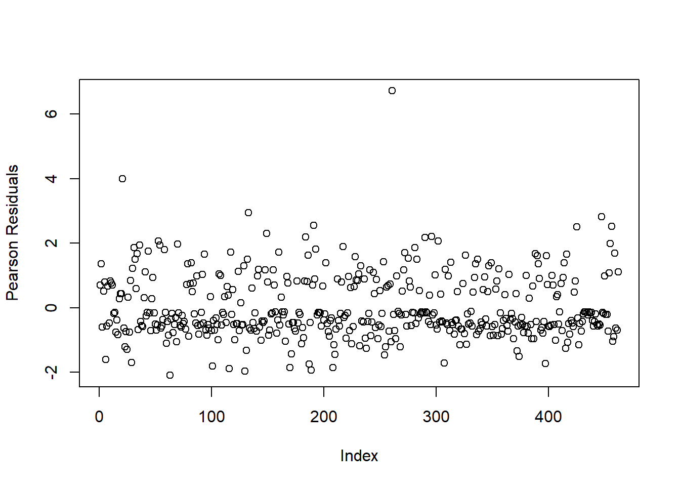
Figure 4.2: Plot of Residuals for Logistic Regression Model
We notice that there are two subjects with high residual values. To identify them, we can use the following code;
# sort residuals largest to smallest and select the first two
sort(residuals(heart_model4, type = "pearson"), decreasing = T)[1:2]
## 261 21
## 6.714401 3.987004Subjects 261 and 21 have high deviance residuals. To see if these are influential observations, we can refit the logistic regression model without these observations. If the estimates of our model change greatly, then we should remove these two observations as they may affect inference and predictions made with the logistic regression model.
Let’s make a second data set without the 261st observation and see if the results of the model change.
heart2 <- heart[-261,] # removing the 261st observation

#fit the model using heart2
heart_model4_2 <- glm(y ~ tobacco + ldl + famhist_f + typea + age_f + ldl*famhist_f,
                    family=binomial(link = "logit"), data=heart2) #use heart2

summary(heart_model4_2) #model summary excluding id 261
##
## Call:
## glm(formula = y ~ tobacco + ldl + famhist_f + typea + age_f +
## ldl * famhist_f, family = binomial(link = "logit"), data = heart2)
##
## Coefficients:
## Estimate Std. Error z value Pr(>|z|)
## (Intercept) -6.41271 1.27032 -5.048 4.46e-07 ***
## tobacco 0.08917 0.02647 3.368 0.000757 ***
## ldl 0.01863 0.07452 0.250 0.802549
## famhist_f1 -0.74549 0.63251 -1.179 0.238552
## typea 0.03743 0.01254 2.985 0.002840 **
## age_f2 2.48866 1.05440 2.360 0.018262 *
## age_f3 2.64455 1.04953 2.520 0.011744 *
## age_f4 2.94108 1.04764 2.807 0.004995 **
## age_f5 3.65866 1.04328 3.507 0.000453 ***
## ldl:famhist_f1 0.33576 0.11769 2.853 0.004332 **
## ---
## Signif. codes: 0 '***' 0.001 '**' 0.01 '*' 0.05 '.' 0.1 ' ' 1
##
## (Dispersion parameter for binomial family taken to be 1)
##
## Null deviance: 593.98 on 460 degrees of freedom
## Residual deviance: 455.17 on 451 degrees of freedom
## AIC: 475.17
##
## Number of Fisher Scoring iterations: 6##
## Call:
## glm(formula = y ~ tobacco + ldl + famhist_f + typea + age_f +
## ldl * famhist_f, family = binomial(link = "logit"), data = heart)
##
## Coefficients:
## Estimate Std. Error z value Pr(>|z|)
## (Intercept) -5.61061 1.04614 -5.363 8.18e-08 ***
## tobacco 0.08901 0.02644 3.366 0.000762 ***
## ldl 0.01087 0.07413 0.147 0.883425
## famhist_f1 -0.81122 0.62828 -1.291 0.196643
## typea 0.03625 0.01243 2.917 0.003535 **
## age_f2 1.79383 0.78263 2.292 0.021902 *
## age_f3 1.95366 0.77616 2.517 0.011834 *
## age_f4 2.24868 0.77355 2.907 0.003650 **
## age_f5 2.96258 0.76746 3.860 0.000113 ***
## ldl:famhist_f1 0.34624 0.11725 2.953 0.003146 **
## ---
## Signif. codes: 0 '***' 0.001 '**' 0.01 '*' 0.05 '.' 0.1 ' ' 1
##
## (Dispersion parameter for binomial family taken to be 1)
##
## Null deviance: 596.11 on 461 degrees of freedom
## Residual deviance: 463.46 on 452 degrees of freedom
## AIC: 483.46
##
## Number of Fisher Scoring iterations: 6We do see that the estimated coefficients and standard errors change after removing the observation. In particular, the estimated regression coefficients and standard errors of the age_f variable changed greatly. This shows that observation 261 is an influential observation, and should be removed.
We can do the same procedure for removing observation 21:
heart3 <- heart[-c(21, 261),] # removing the 21st (and 261st from prev removal)
# observation

#fit the model using heart3
heart_model4_3 <- glm(y ~ tobacco + ldl + famhist_f + typea + age_f + ldl*famhist_f,
                    family=binomial(link = "logit"), data=heart3) #use heart3

summary(heart_model4_3) #model summary excluding id 21 and id 261
##
## Call:
## glm(formula = y ~ tobacco + ldl + famhist_f + typea + age_f +
## ldl * famhist_f, family = binomial(link = "logit"), data = heart3)
##
## Coefficients:
## Estimate Std. Error z value Pr(>|z|)
## (Intercept) -20.65184 793.20342 -0.026 0.979229
## tobacco 0.08771 0.02635 3.328 0.000874 ***
## ldl 0.03073 0.07479 0.411 0.681168
## famhist_f1 -0.65602 0.63603 -1.031 0.302337
## typea 0.03471 0.01254 2.768 0.005642 **
## age_f2 16.82365 793.20311 0.021 0.983078
## age_f3 16.97712 793.20310 0.021 0.982924
## age_f4 17.26763 793.20310 0.022 0.982632
## age_f5 17.97553 793.20309 0.023 0.981920
## ldl:famhist_f1 0.32012 0.11794 2.714 0.006643 **
## ---
## Signif. codes: 0 '***' 0.001 '**' 0.01 '*' 0.05 '.' 0.1 ' ' 1
##
## (Dispersion parameter for binomial family taken to be 1)
##
## Null deviance: 591.85 on 459 degrees of freedom
## Residual deviance: 446.13 on 450 degrees of freedom
## AIC: 466.13
##
## Number of Fisher Scoring iterations: 17##
## Call:
## glm(formula = y ~ tobacco + ldl + famhist_f + typea + age_f +
## ldl * famhist_f, family = binomial(link = "logit"), data = heart)
##
## Coefficients:
## Estimate Std. Error z value Pr(>|z|)
## (Intercept) -5.61061 1.04614 -5.363 8.18e-08 ***
## tobacco 0.08901 0.02644 3.366 0.000762 ***
## ldl 0.01087 0.07413 0.147 0.883425
## famhist_f1 -0.81122 0.62828 -1.291 0.196643
## typea 0.03625 0.01243 2.917 0.003535 **
## age_f2 1.79383 0.78263 2.292 0.021902 *
## age_f3 1.95366 0.77616 2.517 0.011834 *
## age_f4 2.24868 0.77355 2.907 0.003650 **
## age_f5 2.96258 0.76746 3.860 0.000113 ***
## ldl:famhist_f1 0.34624 0.11725 2.953 0.003146 **
## ---
## Signif. codes: 0 '***' 0.001 '**' 0.01 '*' 0.05 '.' 0.1 ' ' 1
##
## (Dispersion parameter for binomial family taken to be 1)
##
## Null deviance: 596.11 on 461 degrees of freedom
## Residual deviance: 463.46 on 452 degrees of freedom
## AIC: 483.46
##
## Number of Fisher Scoring iterations: 6Again we see that the coefficients change significantly and deem the 21st observation to be influential. Thus, we continue our analysis without observation 21 and 261.
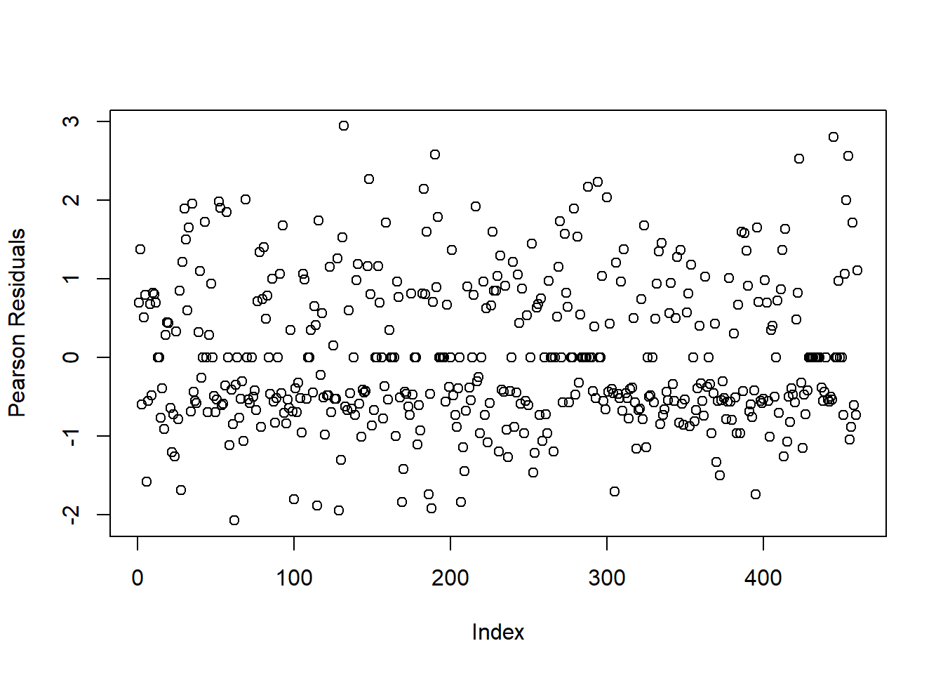
Figure 4.3: Plot of Residuals for Logistic Regression Model with Influential Observation Removed
Now, we see that most residual values fall between \((-2, 2)\) (with no values beyond \(\pm 3\)), which indicates a proper model fit.
We notice that when we look at the model summary, some covariates have very large estimated standard errors and are no longer significant, indicating that after removing the influential observations we should re-do our model fitting.
#fit a full model, including the interaction
heart_full2 <- glm(y ~ sbp + tobacco + ldl + adiposity + famhist_f +
                         typea + obesity + alcohol + age_f + ldl*famhist_f,
                            family=binomial(link = "logit"), data=heart3)


step(heart_full2, direction = "both", trace = 0) #trace = 0 means don't print
##
## Call: glm(formula = y ~ tobacco + ldl + famhist_f + typea + age_f +
## ldl:famhist_f, family = binomial(link = "logit"), data = heart3)
##
## Coefficients:
## (Intercept) tobacco ldl famhist_f1
## -20.65184 0.08771 0.03073 -0.65602
## typea age_f2 age_f3 age_f4
## 0.03471 16.82365 16.97712 17.26763
## age_f5 ldl:famhist_f1
## 17.97553 0.32012
##
## Degrees of Freedom: 459 Total (i.e. Null); 450 Residual
## Null Deviance: 591.9
## Residual Deviance: 446.1 AIC: 466.1Let’s see the summary of the model:
# fit a new model
heart_model6 <- glm(y ~ tobacco + ldl + famhist_f +
                         typea + age_f + ldl*famhist_f ,
                            family=binomial(link = "logit"), data=heart3)
summary(heart_model6)
##
## Call:
## glm(formula = y ~ tobacco + ldl + famhist_f + typea + age_f +
## ldl * famhist_f, family = binomial(link = "logit"), data = heart3)
##
## Coefficients:
## Estimate Std. Error z value Pr(>|z|)
## (Intercept) -20.65184 793.20342 -0.026 0.979229
## tobacco 0.08771 0.02635 3.328 0.000874 ***
## ldl 0.03073 0.07479 0.411 0.681168
## famhist_f1 -0.65602 0.63603 -1.031 0.302337
## typea 0.03471 0.01254 2.768 0.005642 **
## age_f2 16.82365 793.20311 0.021 0.983078
## age_f3 16.97712 793.20310 0.021 0.982924
## age_f4 17.26763 793.20310 0.022 0.982632
## age_f5 17.97553 793.20309 0.023 0.981920
## ldl:famhist_f1 0.32012 0.11794 2.714 0.006643 **
## ---
## Signif. codes: 0 '***' 0.001 '**' 0.01 '*' 0.05 '.' 0.1 ' ' 1
##
## (Dispersion parameter for binomial family taken to be 1)
##
## Null deviance: 591.85 on 459 degrees of freedom
## Residual deviance: 446.13 on 450 degrees of freedom
## AIC: 466.13
##
## Number of Fisher Scoring iterations: 17Although the stepwise procedure (and an LRT) will tell us otherwise, we should remove the age_f variable due to the large, insignificant estimates. It is likely that for this sample, age_f is not adding any value to our model. We refit this model without age_f:
# fit a new model
heart_model7 <- glm(y ~ tobacco + ldl + famhist_f +
                         typea + ldl*famhist_f ,
                            family=binomial(link = "logit"), data=heart3)
summary(heart_model7)
##
## Call:
## glm(formula = y ~ tobacco + ldl + famhist_f + typea + ldl * famhist_f,
## family = binomial(link = "logit"), data = heart3)
##
## Coefficients:
## Estimate Std. Error z value Pr(>|z|)
## (Intercept) -3.47029 0.74548 -4.655 3.24e-06 ***
## tobacco 0.13821 0.02539 5.444 5.22e-08 ***
## ldl 0.09899 0.07189 1.377 0.16850
## famhist_f1 -0.39576 0.61446 -0.644 0.51953
## typea 0.02383 0.01182 2.016 0.04385 *
## ldl:famhist_f1 0.30096 0.11609 2.592 0.00953 **
## ---
## Signif. codes: 0 '***' 0.001 '**' 0.01 '*' 0.05 '.' 0.1 ' ' 1
##
## (Dispersion parameter for binomial family taken to be 1)
##
## Null deviance: 591.85 on 459 degrees of freedom
## Residual deviance: 486.83 on 454 degrees of freedom
## AIC: 498.83
##
## Number of Fisher Scoring iterations: 4and see estimates with less extreme values and variances. When we plot the residuals:
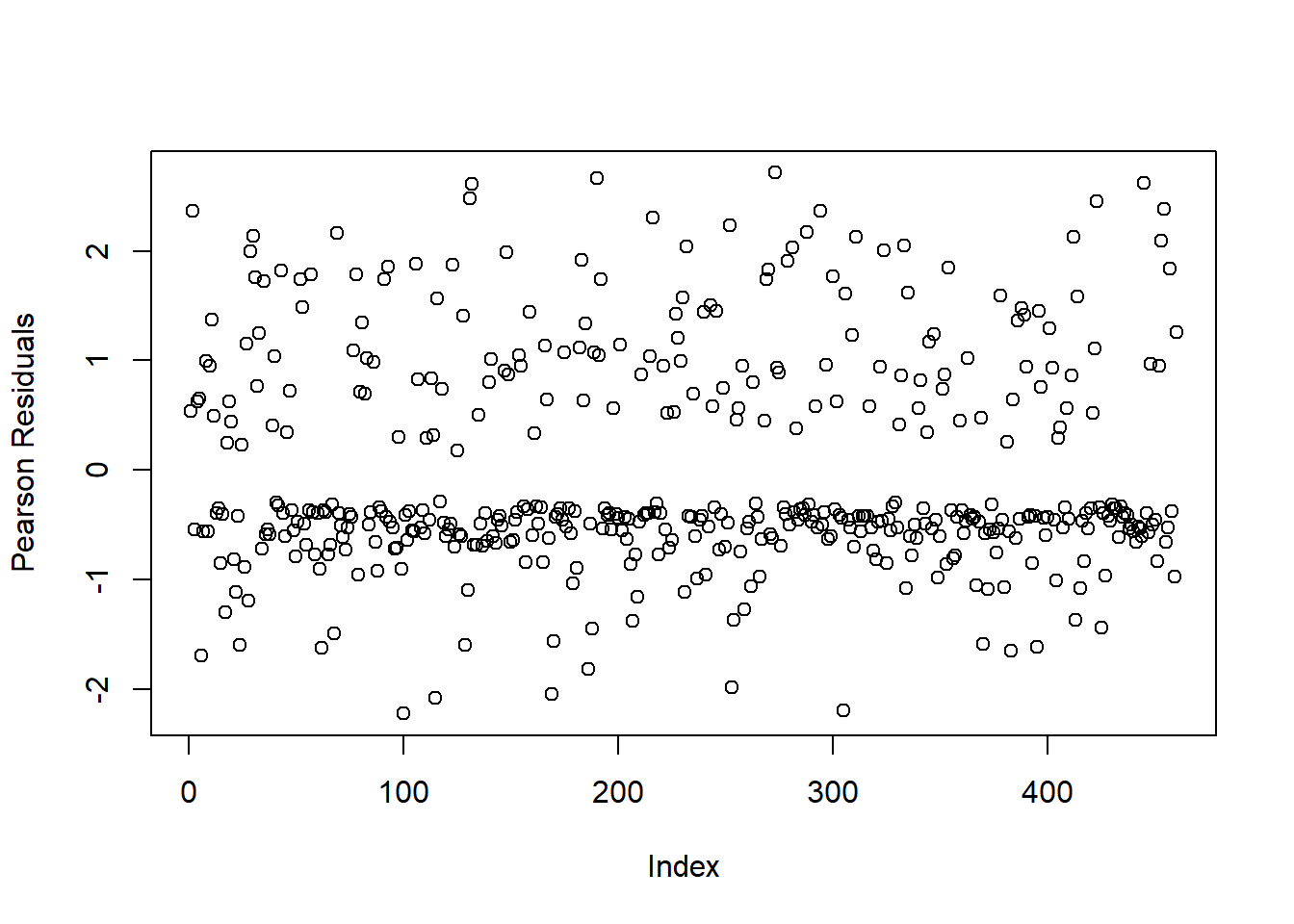
Figure 4.4: Plot of Residuals for Second Regression Modelwith Influential Observation Removed
We see that the residuals are behaving as expected with no extreme values.
We should also check for multicollinearity in our model. We can do so by using the vif() function from the car package. We can do so by the following R code:
# there are multiple vif functions so car:: specifies
# we are using the vif function from the car package
car::vif(heart_model7) ## tobacco ldl famhist_f typea
## 1.034016 1.649904 7.596317 1.013287
## ldl:famhist_f
## 8.480374We see that we only have low-moderate variance inflation factors (VIFs), indicating that multicollinearity is not an issue in this model. We typically are concerned about multicollinearity when VIF values are above 10.
4.6.1.3 Model Interpretation and Hypothesis Testing
Odds Ratios
As previously mentioned, we interpret each coefficients as the log odds ratio of the outcome for a one unit change in the corresponding covariate, controlling for the other covariates in the model. That means, to obtain estimates of the odds ratio, we take the exponential (exp() in R) of the coefficient. The estimates of the standard error for the coefficients (log-odds) will be useful for hypothesis testing and constructing confidence intervals.
Let’s look again at the model we chose from the selection procedure:
##
## Call:
## glm(formula = y ~ tobacco + ldl + famhist_f + typea + ldl * famhist_f,
##     family = binomial(link = "logit"), data = heart3)
##
## Coefficients:
##                Estimate Std. Error z value Pr(>|z|)
## (Intercept)    -3.47029    0.74548  -4.655 3.24e-06 ***
## tobacco         0.13821    0.02539   5.444 5.22e-08 ***
## ldl             0.09899    0.07189   1.377  0.16850
## famhist_f1     -0.39576    0.61446  -0.644  0.51953
## typea           0.02383    0.01182   2.016  0.04385 *
## ldl:famhist_f1  0.30096    0.11609   2.592  0.00953 **
## ---
## Signif. codes:  0 '***' 0.001 '**' 0.01 '*' 0.05 '.' 0.1 ' ' 1
##
## (Dispersion parameter for binomial family taken to be 1)
##
##     Null deviance: 591.85  on 459  degrees of freedom
## Residual deviance: 486.83  on 454  degrees of freedom
## AIC: 498.83
##
## Number of Fisher Scoring iterations: 4In mathematical notation, we can write this model as
\[ \begin{aligned} \text{log} \left[\frac{\pi_i}{1-\pi_i} \right]= \beta_0 + &\beta_1x_1 + \beta_2x_2 + \beta_3x_3 + \beta_4x_4 + \beta_5x_2*x_3 \end{aligned} \] where \(\pi_i\) is the probability of having CHD, \(x_1\) is the measurement of cumulative tobacco use, \(x_2\) is the ldl cholesterol measurement, \(x_3\) is an indicator for family history, and \(x_4\) is the type a measurement.
We are provided with the estimates and standard errors of the log odds ratios, but typically want to interpret and communicate our findings on the scale of odd ratios. To obtain an estimate of the odds ratio for a given covariate, we simply exponentiate the coefficient. For example, the tobacco covariate’s estimated coefficient (\(\widehat{\beta_1}\)) is 0.138, meaning we estimate that a one unit increase in tobacco is associated with a log odds ratio of chronic heart disease equal to 0.138, controlling for the other factors in the model. Alternatively, we can say that a one unit increase in tobacco is associated with an odds ratio of chronic heart disease equal to \(\exp(\) 0.138 \()\) = 1.148, controlling for other factors.
Confidence intervals (CIs) are useful in communicating the uncertainty in our estimates and are typically presented along with our estimate. Confidence intervals are calculated on the log odds ratio scale, and then exponentiated to find the confidence interval for the odds ratio. We calculate a 95% confidence interval for a log odds ratio as:
\[
\widehat{\beta} \pm 1.96\times \widehat{se}(\widehat{\beta})
\]
where \(\widehat{se}(\widehat{\beta})\) is the estimated standard error of the regression coefficient. For example, a 95% confidence interval for the log odds ratio of tobacco is
\[
0.138 \pm 1.960 \times 0.025 = (0.089, 0.187).
\]
Then, to find the 95% CI for the odds ratio, we exponentiate both sides of the CI as:
\[
(\exp(0.089), \exp(0.187)) = (1.093, 1.206)
\]
So, we estimate the odds ratio to be 1.148 (95% CI: (1.093, 1.206)) controlling for the other factors in the model. As this 95% CI does not contain the value of OR = 1 in it, we say that we are 95% confident that higher tobacco use is associated with an increased odds of developing CHD.
For the odds ratios and confidence intervals of the regression coefficients individually, one can also call the confint.default() function
logORs <- cbind(coef(heart_model7), confint.default(heart_model7))
colnames(logORs) <- c("logOR", "Lower", "Upper")
logORs
## logOR Lower Upper
## (Intercept) -3.47028789 -4.9314011158 -2.00917466
## tobacco 0.13820940 0.0884465653 0.18797224
## ldl 0.09899415 -0.0419048152 0.23989312
## famhist_f1 -0.39575571 -1.6000802163 0.80856880
## typea 0.02382659 0.0006571497 0.04699603
## ldl:famhist_f1 0.30095626 0.0734244303 0.52848808and exponentiate it to get the ORs:
##                Odds Ratio       Lower     Upper
## (Intercept)    0.03110807 0.007216385 0.1340993
## tobacco        1.14821596 1.092475875 1.2068000
## ldl            1.10405984 0.958961055 1.2711133
## famhist_f1     0.67317113 0.201880323 2.2446931
## typea          1.02411271 1.000657366 1.0481178
## ldl:famhist_f1 1.35115024 1.076187206 1.6963656
For another example, let’s look at estimating the odds ratio of CHD for a one unit increase in ldl among those with a family history of CHD, controlling for the other factors. For more complex estimates where we may be interested in combinations of covariates, it can be useful to create a table to determine what regression coefficients we want to use.
Recall the model
\[
\begin{aligned}
\text{log} \left[\frac{\pi_i}{1-\pi_i} \right]= \beta_0 + &\beta_1x_1 + \beta_2x_2 + \beta_3x_3 + \beta_4x_4 + \beta_5x_2x_3.
\end{aligned}
\]
and recall \(x_2\) represents ldl and \(x_3\) represents famhist_f.
We wish to estimate the odds ratio of CHD for a one unit increase in ldl, which is the same as looking at \(x_2\) = 1 versus \(x_2 = 0\) (or \(x_2 = 2\) versus \(x_2 = 1\), and so on, however 1 versus 0 is the simplest example). We also are interested in only those with a family history of CHD, represented by \(x_3 = 1\). All of the other covariates are held constant. So, we are comparing
\[ \begin{aligned} \beta_0 + &\beta_1x_1 + \beta_2(1) + \beta_3(1) + \beta_4x_4 + \beta_5(1)(1) \end{aligned} \] to \[ \begin{aligned} \beta_0 + &\beta_1x_1 + \beta_2(0) + \beta_3(1) + \beta_4x_4 + \beta_5(0)(1) \end{aligned} \] If we look at the difference of these equations, we have \[ \begin{aligned} & \beta_0 + \beta_1x_1 + \beta_2(1) + \beta_3(1) + \beta_4x_4 + \beta_5(1)(1)\\ &-\left(\beta_0 + \beta_1x_1 + \beta_2(0) + \beta_3(1) + \beta_4x_4 + \beta_5(0)(1)\right)\\ \hline & \qquad \qquad \qquad \quad \beta_2 \qquad \quad \quad \quad \qquad \quad+\beta_5 \end{aligned} \] which shows that we should estimate and interpret \(\beta_2 + \beta_5\) to answer this question. From the model output, we estimate the log odds ratio as \(\widehat{\beta_2} + \widehat{\beta_5} = 0.099 + 0.301 = 0.400\). Then, the estimated odds ratio is \(\exp(0.400) = 1.492\). So, we estimate that a one unit increase in low density lipoprotein cholesterol is associated with an odds ratio of CHD equal to 1.492, controlling for other factors.
To estimate the confidence interval, we must find the estimated standard error of \(\widehat{\beta_2} + \widehat{\beta_5}\) manually, construct a confidence interval for this quantity (the logOR), and then exponentiate each bound of the confidence interval. To do so in R, we can use the following code:
varcov <- vcov(heart_model7) #get the variance covariance matrix
L <- c(0, 0, 1, 0, 0, 1) #represents \beta_2 + \beta_5 (first place is beta_0)

var_est <- L%*%varcov %*% L
beta_est <- L%*%coef(heart_model7) #vector of coefficients from model

CI <- c(beta_est - 1.96*sqrt(var_est), beta_est + 1.96*sqrt(var_est))

exp(CI) #exponentiate to get CI for OR
## [1] 1.247937 1.783199Probabilities
Perhaps we are interested in estimating or predicting the probability of the outcome instead of the odds ratio for given covariates.
Suppose we are interested in the probability that a 25 year old with spb = 150, tobacco = 0, ldl = 6, adiposity = 24, no family history of CHD, typea = 60, obesity = 30, and alcohol = 10. Using the required information, we can obtain a prediction using the predict() function as:
# make a vector of the new information as it would appear in the original
# dataframe (excluding y). Use colnames(heart) to see the order of variables
newsubject <- data.frame(sbp = 150,
                         tobacco = 0,
                         ldl = 6,
                         adiposity = 24,
                         famhist = 0,
                         typea = 60,
                         obesity = 30,
                         alcohol = 10,
                         age = 25,
                         age_f = 2,
                         famhist_f = 1
                         )

newsubject$age_f <- as.factor(newsubject$age_f)
newsubject$famhist_f <- as.factor(newsubject$famhist_f)

predict(heart_model7, newdata = newsubject)
## 1
## -0.03674586We estimate that \(\frac{\log{\pi}}{1 - \pi} = -0.037\). So, to estimate the probability, we take the expit() of this estimate, or obtain \[ \frac{\exp(-0.037)}{1 + \exp(-0.037)} = 0.491 \] We estimate this hypothetical individual to have a 49.1% probability of having CHD given their covariates.
4.7 Binominal Distributed/Proportional Outcomes (Logistic Regression on Proportions)
Sometimes when evaluating a binary response, we don’t have data for each individual in the study and cannot fit a logistic regression in the usual way. However, if we have the proportion of outcomes for various subgroups in our data set, we can still model the proportion of outcomes using a binomial generalized linear model. That is, we observe \(y_j/m_j\) for each combination \(j = 1, 2, ..., J\) of our variables \(\boldsymbol{x}\) where \(y_j\) is the number of successes/occurrences in a subgroup \(j\) of size \(m_j\). We note that this method is recommended over treating the proportion as a continuous outcome and fitting a linear regression model. This is because the proportions may not be normally distributed, or even continuous for small \(m\).
We model the expected proportions as a function of the covariates of interest using a binomial regression model (logistic regression). We can fit a generalized linear model two ways: we can either model the response as a pair where the response is cbind(y, m - y) or model the response as y/m where we set weights = m as a parameter in the glm() function. In both settings, we let family = binomial() and specify a link function.
The following example shows the use of the binomial regression model, and explains how we can fit the model in two different ways.
4.7.1 Example
We will be looking at a data set involving the proportions of children who have reached menarche at different ages. The data set contains the average age of the group (which are reasonably homogeneous) (Age), the total number of children in the group (Total), and the number of children in the group who have reached menarche (Menarche). The goal of this analysis is to see quantify the relationship between age and menarche onset. We first load the menarche data set from the MASS package:
# load the data from MASS package
data("menarche")

# look at first 6 observations of the data
head(menarche)
## Age Total Menarche
## 1 9.21 376 0
## 2 10.21 200 0
## 3 10.58 93 0
## 4 10.83 120 2
## 5 11.08 90 2
## 6 11.33 88 5We see that for different age groups, we have different sizes of the number of individuals in that group (Total), and the corresponding number of children who have reached menarche (Menarche). The proportion of people who have reached menarche in each age group is then Menarche/Total.
4.7.1.1 Model Fitting
Recall that we can fit a model two ways: fitting the outcome as cbind(y, m - y) or fitting the outcome as y/m where we set weights = m as a parameter in the glm() function. We will show that these models produce the same results. We will fit both models using the canonical logit link. First, we fit the model using the paired response:
menarche_fit1 <- glm(cbind(Menarche, Total - Menarche) ~ Age,
                     data = menarche,
                     family = binomial(link = "logit"))

summary(menarche_fit1)
##
## Call:
## glm(formula = cbind(Menarche, Total - Menarche) ~ Age, family = binomial(link = "logit"),
## data = menarche)
##
## Coefficients:
## Estimate Std. Error z value Pr(>|z|)
## (Intercept) -21.22639 0.77068 -27.54 <2e-16 ***
## Age 1.63197 0.05895 27.68 <2e-16 ***
## ---
## Signif. codes: 0 '***' 0.001 '**' 0.01 '*' 0.05 '.' 0.1 ' ' 1
##
## (Dispersion parameter for binomial family taken to be 1)
##
## Null deviance: 3693.884 on 24 degrees of freedom
## Residual deviance: 26.703 on 23 degrees of freedom
## AIC: 114.76
##
## Number of Fisher Scoring iterations: 4Next, we fit the model using the proportions and specifying the weights:
menarche_fit2 <- glm(Menarche/Total ~ Age,
                     data = menarche,
                     weights = Total,
                     family = binomial(link = "logit"))

summary(menarche_fit2)
##
## Call:
## glm(formula = Menarche/Total ~ Age, family = binomial(link = "logit"),
## data = menarche, weights = Total)
##
## Coefficients:
## Estimate Std. Error z value Pr(>|z|)
## (Intercept) -21.22639 0.77068 -27.54 <2e-16 ***
## Age 1.63197 0.05895 27.68 <2e-16 ***
## ---
## Signif. codes: 0 '***' 0.001 '**' 0.01 '*' 0.05 '.' 0.1 ' ' 1
##
## (Dispersion parameter for binomial family taken to be 1)
##
## Null deviance: 3693.884 on 24 degrees of freedom
## Residual deviance: 26.703 on 23 degrees of freedom
## AIC: 114.76
##
## Number of Fisher Scoring iterations: 4We see that these models are equivalent.
4.7.1.2 Model Diagnostics
We can look at the model fit by evaluating the residual and fitted values:
# first plot the residual vs dose
resid_menarche <- residuals.glm(menarche_fit1, "deviance")
plot(menarche$Age, resid_menarche, ylim = c(-3, 3),
     main = "Deviance Residuals vs Age",
     ylab = "Residuals",
     xlab = "Age")
abline(h = -2, lty = 2) # add dotted lines at 2 and -2
abline(h = 2, lty = 2)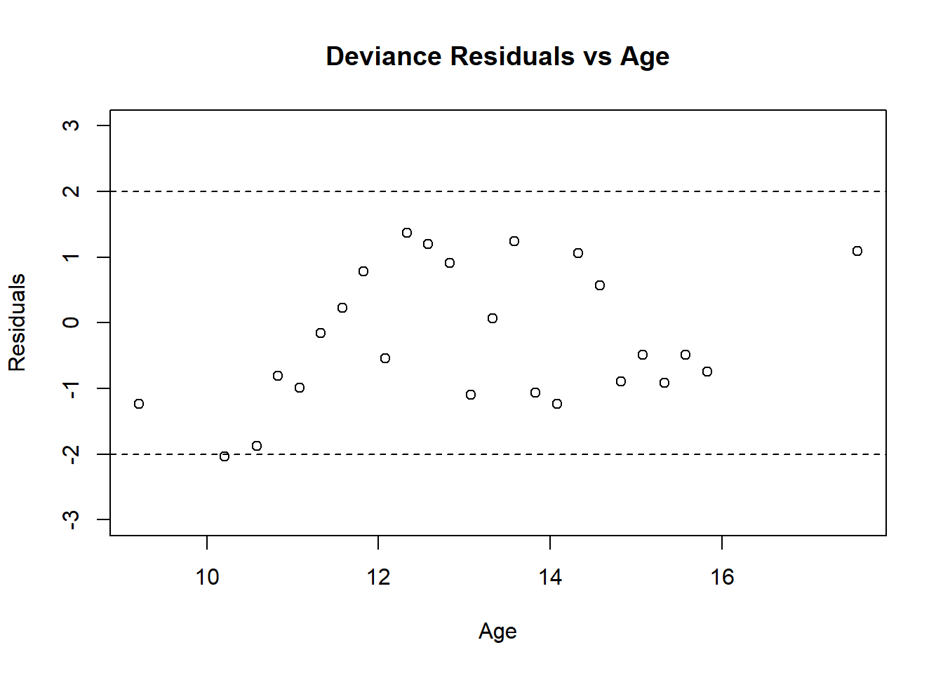
Figure 4.5: Residual plot for Menarche GLM
# then plot the fitted versus dose
fitted_menarche <- menarche_fit1$fitted.values
plot(menarche$Age, fitted_menarche, ylim = c(0, 1),
     main = "Fitted Value vs Age",
     ylab = "Probability of Menarche",
     xlab = "Age",
     pch = 19)
points(menarche$Age, menarche$Menarche/menarche$Total, col = "red", pch = 8)
legend(13, 0.3, legend = c("Fitted", "Observed"), col = c("black", "red"), pch = c(19, 8))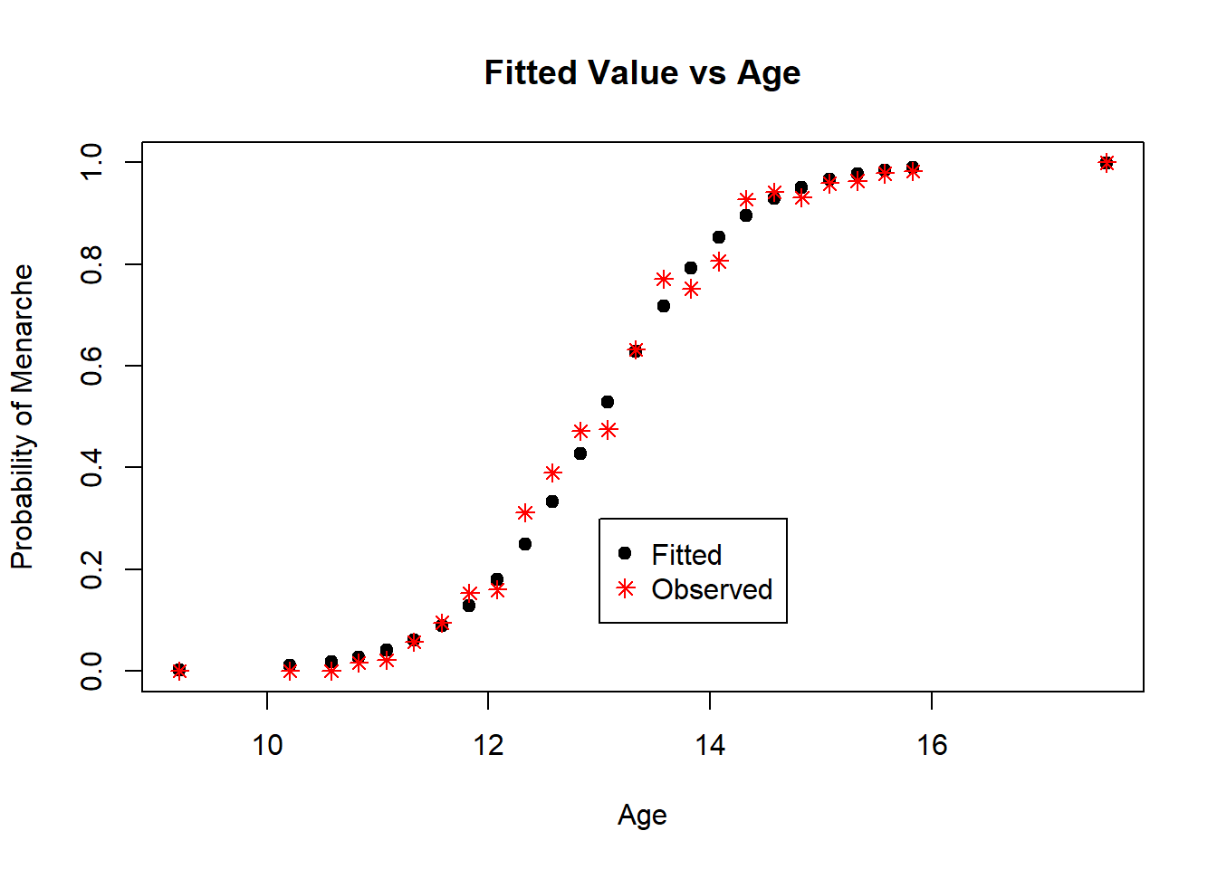
Figure 4.6: Diagnostic Plot for Probit Model: Fitted Values
The residuals in Figure 4.5 are mostly between -2 and 2, and show no signs of a poor fit. The plot of the fitted and observed values in Figure 4.6 are similar, indicating good prediction for the observations we fit our model on. Overall, this model appears to be a good fit for the data.
4.7.1.3 Model Interpretation
From (either) model output, we see that age is significantly associated with menarche. As we used the logit link, the interpretation of our parameters are log odds ratios. As such, we can interpret the model output as follows:
- \(\beta_0\): At age = 0, the log odds of menarche is estimated to be -21.226 (the odds is estimated to be \(\exp(-21.226)\) = 0.000). This makes sense in the context of our study.
- \(\beta_1\): For a one unit increase in the average age, we estimate the log odds of menarche to be 1.632 times higher (the odds ratio is estimated to be \(\exp(1.632)\) = 5.114 times higher). Confidence intervals can be calculated as in Section 4.6.
From these results, we conclude that age is significantly associated with menarche onset.
We can also estimate the probability of menarche onset for certain ages. For example, let’s estimate the probability of menarche for a 13 year old child based on this model. Our model is \[ \log\left(\frac{\widehat{\pi}_i}{1 - \widehat{\pi}}_i\right) = -21.226 + 1.632*\text{Age}_i \] which we can re-write as \[ \widehat{\pi}_i = \frac{\exp(-21.226 + 1.632*\text{Age}_i)}{1 + \exp(-21.226 + 1.632*\text{Age}_i)}. \] Thus, at age 13, we can estimate the probability of menarche as \[ \widehat{\pi}_i = \frac{\exp(-21.226 + 1.632*13)}{1 + \exp(-21.226 + 1.632*13)}. \] We can calculate this by hand, or use the following commands in R:
# grab the coefficients of the model
est_beta <- menarche_fit1$coefficients #beta[1] is the intercept,
# beta[2] is the coefficient on age


# estimate the probability
est_prob <- exp(est_beta[1] + est_beta[2]*13)/(1 + exp(est_beta[1] + est_beta[2]*13))
print(paste("Estimated probability:", round(est_prob,3))) #print it out, rounded
## [1] "Estimated probability: 0.497"Thus, for a 13 year old child, we estimate the probability of menarche to be 49.7%.
4.7.2 Dose-response Models
Suppose we want to quantify a dose-response relationship between a stimulus (dose) and a particular outcome (response). We typically see dose-response relationships in bioassay experiments where we expose groups of living subjects to varying doses of a toxin and determine how many deaths or other binary health outcomes there are within a given time period. Given the concentration of the toxin, we calculate the dose as
\[ x = \text{dose} = \log(\text{concentration}) \] We assume that for each subject in the bioassay study there is a tolerance or threshold dosage where a response will always occur. This value can vary from individual to individual and can be described by a statistical distribution. For each group \(j = 1, 2, \dots, J\), we let \(m_j\) be the total number of subjects in group \(j\), \(x_j\) be the dose applied to all subjects in group \(i\), and \(y_i\) be the number of subjects that responded in group \(j\).
We assume that \(Y_j\) follows a binomial distribution with \(n\) = \(m_j\) and unknown probability of response \(\pi_j\). We can model this using a GLM as \[ g(\pi) = \beta_0 + \beta_1x \] where \(g()\) is a link function.
Choices of \(g()\) include the probit, logit, and complimentary log-log (cloglog). The “best” link function depends on the underlying distribution of the probability \(\pi\). After describing the link functions, we will show in an example in Section 4.7.2.1 that includes how to choose the link function from the data.
Probit Link
If \(\pi(x)\) is normally distributed, use probit link \(g(\pi) = \Phi^{-1}(\pi)\) where \(\Phi\) is the standard normal distribution CDF (cumulative distribution function)
Using this link function, we do not have the interpretation of odds ratios as we are not using the logistic link function. We can re-write the relationship between \(\pi\) and the covariate \(x\) through the link function as \[ \pi(x) = g^{-1}(\beta_0 + \beta_1x) = \Phi\left( \frac{x - \mu}{\sigma} \right) \] where \(\mu\) is the mean and \(\sigma\) is the standard deviation of the tolerance distribution (here we subtract the mean and divide by the standard deviation to create a standard normal distribution).
We may be the median lethal/effective dose at which 50% of the population has a response (\(\delta_{0.5}\)), which is calculated as \[ \delta_{0.5} = \frac{-\beta_0}{\beta_1} \]
which can be calculated using the GLM model output. We can also obtain expressions for the 100\(p\)th percentile of the tolerance distribution (\(\delta_p\)) as \[ \delta_p = \frac{\Phi^{-1}(p) - \beta_0}{\beta_1} \] where \(\Phi^{-1}()\) is the inverse of the standard normal CDF.
Logit Link
If we assume the probability has the form \(\pi(x) = \frac{\exp(\beta_0 + \beta_1x)}{1 + \exp(\beta_0 + \beta_1x)}\), then we can use the logit link \(g(\pi) = \log\left(\frac{\pi}{1 - \pi}\right)\). We interpret the parameters \(\beta_0\) and \(\beta_1\) as log odds/log odds ratios as in our “usual” logistic regression. That is, \(\beta_0\) is the log odds of response for a dose of zero and \(\beta_1\) is the log odds ratio for response associated with a one unit increase in the dose. To find odds/odds ratios, we exponentiate the coefficients.
The median lethal/effective dose is the same as the probit link, which is \[ \delta_{0.5} = \frac{-\beta_0}{\beta_1}. \] It is also possible to obtain expressions for any percentile of the tolerance distribution. That is, the 100\(p\)th percentile of the tolerance distribution for \((0 < p < 1)\) can be found by solving \[ \log{\frac{p}{1-p}} = \beta_0 + \beta_1\delta_p \] where \(\delta_p\) is the dosage we’d like to solve for.
Complimentary Log-log Link
If we assume \(\pi(x) = 1 - \exp(-\exp(\beta_0 + \beta_1x))\) (extreme value distribution), we can use the complementary log-log (cloglog) link \(g(\pi) = \log(-\log(1 - \pi))\)
The interpretation of the parameters when using a complimentary log-log link function is not as “nice” as when using the logit or probit links, however we can still obtain an expression for the median lethal/effective dose, which is \[ \delta_{0.5} = \frac{\log(-\log(1 - 0.5)) - \beta_0}{\beta_1}. \]
4.7.2.1 Example
We use data from a study by (Milesi, Pocquet, and Labbé 2013) to evaluate the dose-response relationship of insecticide dosages and insect fatalities. We will focus on one particular strain of insecticide for the first replicate of the study.
To read in this data, which is located in the “data” folder, we perform the following:
# read in the data
insecticide <- read.table("data/insectdoseresponse.txt", header = T)

# change colnames to english
colnames(insecticide) <- c("insecticide", "strain", "dose", "m", "deaths",
                           "replicate", "date", "color")

# view first 6 observations
head(insecticide)
## insecticide strain dose m deaths replicate date color
## 1 temephos KIS-ref 0.000 100 1 1 26/01/11 1
## 2 temephos KIS-ref 0.002 97 47 1 26/01/11 1
## 3 temephos KIS-ref 0.003 96 68 1 26/01/11 1
## 4 temephos KIS-ref 0.004 98 89 1 26/01/11 1
## 5 temephos KIS-ref 0.005 95 90 1 26/01/11 1
## 6 temephos KIS-ref 0.007 99 97 1 26/01/11 1We are only interested in a subset of this data for the purposes of this example. We are only interested in the first replication of the KIS-ref strain. As such, we subset the data by:
# only keep rows where souche == KIS-ref and replicate = 1
insecticide <- insecticide[insecticide$strain == "KIS-ref" & insecticide$replicate == 1, ]
insecticide
## insecticide strain dose m deaths replicate date color
## 1 temephos KIS-ref 0.000 100 1 1 26/01/11 1
## 2 temephos KIS-ref 0.002 97 47 1 26/01/11 1
## 3 temephos KIS-ref 0.003 96 68 1 26/01/11 1
## 4 temephos KIS-ref 0.004 98 89 1 26/01/11 1
## 5 temephos KIS-ref 0.005 95 90 1 26/01/11 1
## 6 temephos KIS-ref 0.007 99 97 1 26/01/11 1
## 7 temephos KIS-ref 0.010 99 99 1 26/01/11 1To fit a dose-response GLM to this data, we need to have the total number of insects in each group, the dose (log(concentration)), and construct the appropriate paired response variable for the regression (y, m - y). In this data set, we already have the dose (dose) and number of events (deaths) and group totals (m). Prior to fitting the glm, we just need to construct the response variable. To do so in R, we perform the following:
# calculate response variable
insecticide$response <- cbind(insecticide$deaths, insecticide$m - insecticide$deaths)

# look at the data
insecticide
## insecticide strain dose m deaths replicate date color
## 1 temephos KIS-ref 0.000 100 1 1 26/01/11 1
## 2 temephos KIS-ref 0.002 97 47 1 26/01/11 1
## 3 temephos KIS-ref 0.003 96 68 1 26/01/11 1
## 4 temephos KIS-ref 0.004 98 89 1 26/01/11 1
## 5 temephos KIS-ref 0.005 95 90 1 26/01/11 1
## 6 temephos KIS-ref 0.007 99 97 1 26/01/11 1
## 7 temephos KIS-ref 0.010 99 99 1 26/01/11 1
## response.1 response.2
## 1 1 99
## 2 47 50
## 3 68 28
## 4 89 9
## 5 90 5
## 6 97 2
## 7 99 0We will fit three models, one with each of the previously discussed link functions, using the glm() function. We start with the probit link:
# fit the glm using link = "probit"
insecticide_fit_probit <- glm(response ~ dose,
                              family = binomial(link = "probit"), data = insecticide)

# look at the model output
summary(insecticide_fit_probit)
##
## Call:
## glm(formula = response ~ dose, family = binomial(link = "probit"),
## data = insecticide)
##
## Coefficients:
## Estimate Std. Error z value Pr(>|z|)
## (Intercept) -1.5102 0.1508 -10.02 <2e-16 ***
## dose 658.3608 49.5291 13.29 <2e-16 ***
## ---
## Signif. codes: 0 '***' 0.001 '**' 0.01 '*' 0.05 '.' 0.1 ' ' 1
##
## (Dispersion parameter for binomial family taken to be 1)
##
## Null deviance: 433.593 on 6 degrees of freedom
## Residual deviance: 19.862 on 5 degrees of freedom
## AIC: 45.692
##
## Number of Fisher Scoring iterations: 6# assess the residuals
# first plot the residual vs dose
resid_probit <- residuals.glm(insecticide_fit_probit, "deviance")
plot(insecticide$dose, resid_probit, ylim = c(-3, 3),
main = "Deviance Residuals vs Dose: Probit",
ylab = "Residuals",
xlab = "Dose")
abline(h = -2, lty = 2) # add dotted lines at 2 and -2
abline(h = 2, lty = 2)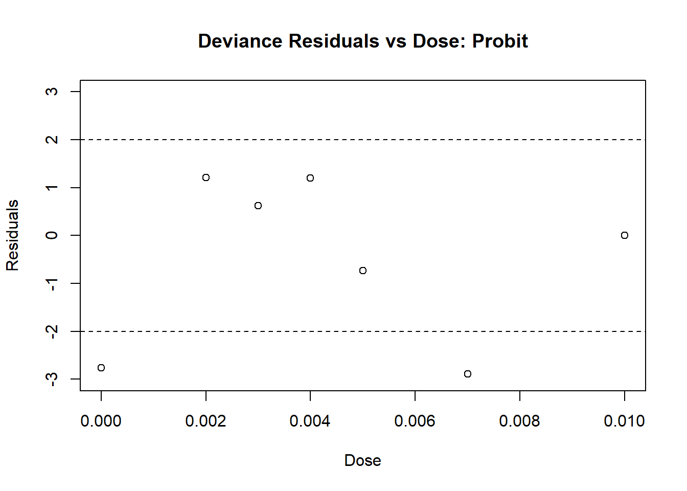
Figure 4.7: Diagnostic Plot for Probit Model: Residuals
# then plot the fitted versus dose
fitted_probit <- insecticide_fit_probit$fitted.values
plot(insecticide$dose, fitted_probit, ylim = c(0, 1),
     main = "Fitted Value vs Dose: Probit Model",
     ylab = "Probability of Death",
     xlab = "Dose",
     pch = 19)
points(insecticide$dose, insecticide$deaths/insecticide$m,
       col = "red", pch = 8)
legend(0.008, 0.3, legend = c("Fitted", "Observed"),
       col = c("black", "red"), pch = c(19, 8))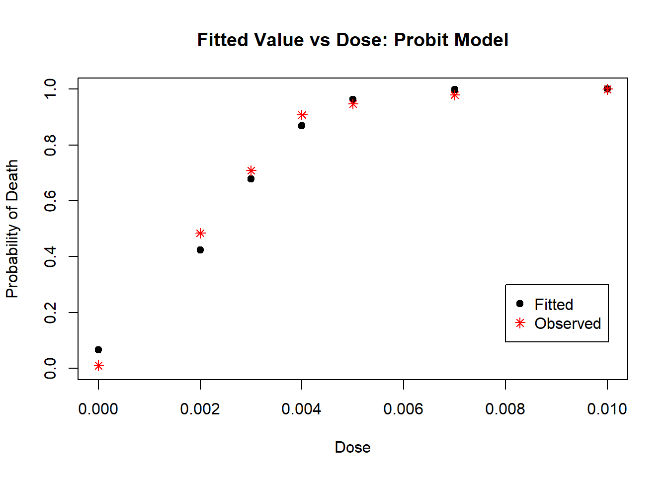
Figure 4.8: Diagnostic Plot for Probit Model: Fitted Values
From Plots 4.7 we see that most residuals fall within (-2, 2), which we would expect for a model with an adequate fit. From Plot 4.8, the fitted values mostly agree with the observed values, with no large deviations.
Next, we can fit the model using a logit link:
# fit the glm using link = "logit"
insecticide_fit_logit <- glm(response ~ dose,
                             family = binomial(link = "logit"), data = insecticide)

# look at the model output
summary(insecticide_fit_logit)
##
## Call:
## glm(formula = response ~ dose, family = binomial(link = "logit"),
## data = insecticide)
##
## Coefficients:
## Estimate Std. Error z value Pr(>|z|)
## (Intercept) -2.7636 0.3006 -9.195 <2e-16 ***
## dose 1215.5565 103.6385 11.729 <2e-16 ***
## ---
## Signif. codes: 0 '***' 0.001 '**' 0.01 '*' 0.05 '.' 0.1 ' ' 1
##
## (Dispersion parameter for binomial family taken to be 1)
##
## Null deviance: 433.593 on 6 degrees of freedom
## Residual deviance: 13.457 on 5 degrees of freedom
## AIC: 39.287
##
## Number of Fisher Scoring iterations: 5# assess the residuals
# first plot the residual vs dose
resid_logit <- residuals.glm(insecticide_fit_logit, "deviance")
plot(insecticide$dose, resid_logit, ylim = c(-3, 3),
main = "Deviance Residuals vs Dose: logit",
ylab = "Residuals",
xlab = "Dose")
abline(h = -2, lty = 2) # add dotted lines at 2 and -2
abline(h = 2, lty = 2)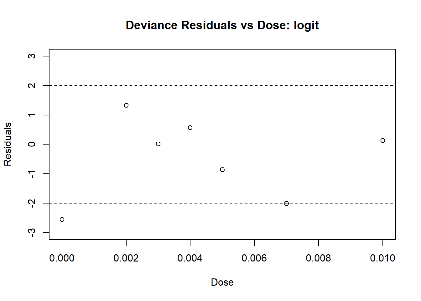
Figure 4.9: Diagnostic Plot for logit Model: Residuals
# then plot the fitted versus dose
fitted_logit <- insecticide_fit_logit$fitted.values
plot(insecticide$dose, fitted_logit, ylim = c(0, 1),
main = "Fitted Value vs Dose: logit Model",
ylab = "Probability of Death",
xlab = "Dose",
pch = 19)
points(insecticide$dose, insecticide$deaths/insecticide$m,
col = "red", pch = 8)
legend(0.008, 0.3, legend = c("Fitted", "Observed"),
col = c("black", "red"), pch = c(19, 8))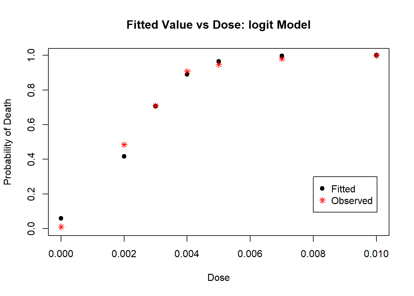
Figure 4.10: Diagnostic Plot for logit Model: Fitted Values
From Plots 4.9 we see that most residuals fall within (-2, 2), which we would expect for a model with an adequate fit. From Plot 4.10, the fitted values mostly agree with the observed values, with no large deviations. This model is very similar to the one with the probit link model.
Next, we fit the model using the complimentary log-log link:
# fit the glm using link = "cloglog"
insecticide_fit_cloglog <- glm(response ~ dose,
family = binomial(link = "cloglog"), data = insecticide)## Warning: glm.fit: fitted probabilities numerically 0 or 1 occurred##
## Call:
## glm(formula = response ~ dose, family = binomial(link = "cloglog"),
## data = insecticide)
##
## Coefficients:
## Estimate Std. Error z value Pr(>|z|)
## (Intercept) -1.6246 0.1686 -9.633 <2e-16 ***
## dose 540.3020 47.1056 11.470 <2e-16 ***
## ---
## Signif. codes: 0 '***' 0.001 '**' 0.01 '*' 0.05 '.' 0.1 ' ' 1
##
## (Dispersion parameter for binomial family taken to be 1)
##
## Null deviance: 433.593 on 6 degrees of freedom
## Residual deviance: 55.806 on 5 degrees of freedom
## AIC: 81.636
##
## Number of Fisher Scoring iterations: 16# assess the residuals
# first plot the residual vs dose
resid_cloglog <- residuals.glm(insecticide_fit_cloglog, "deviance")
plot(insecticide$dose, resid_cloglog, ylim = c(-6, 4),
main = "Deviance Residuals vs Dose: cloglog",
ylab = "Residuals",
xlab = "Dose")
abline(h = -2, lty = 2) # add dotted lines at 2 and -2
abline(h = 2, lty = 2)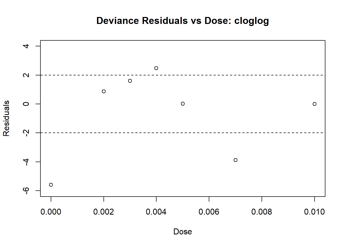
Figure 4.11: Diagnostic Plot for cloglog Model: Residuals
# then plot the fitted versus dose
fitted_cloglog <- insecticide_fit_cloglog$fitted.values
plot(insecticide$dose, fitted_cloglog, ylim = c(0, 1),
main = "Fitted Value vs Dose: cloglog Model",
ylab = "Probability of Death",
xlab = "Dose",
pch = 19)
points(insecticide$dose, insecticide$deaths/insecticide$m,
col = "red", pch = 8)
legend(0.008, 0.3, legend = c("Fitted", "Observed"),
col = c("black", "red"), pch = c(19, 8))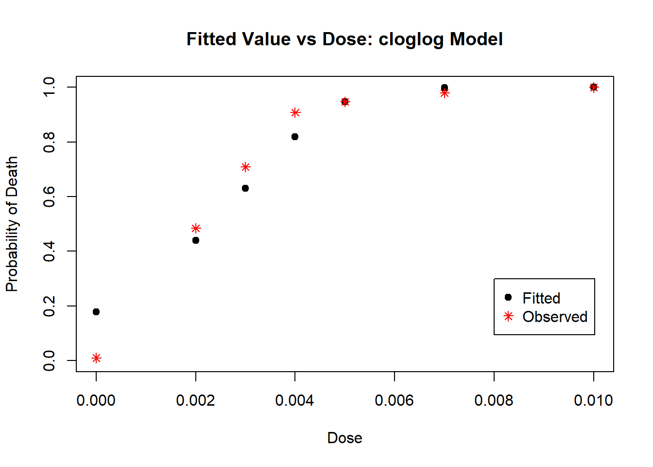
Figure 4.12: Diagnostic Plot for cloglog Model: Fitted Values
From Plots 4.11 we some very large residuals, indicating an inadequate fit. From Plot 4.12, the fitted values do not agree with the observed values, with some large deviations. From these three models, it appears that the logit or probit models are the best.
We can plot the entire dose/response curve from the logit and probit models using the following code:
x = seq(0, 0.010, by = 0.0001) # tiny increments over the doses
prob_logit = as.vector(rep(1, length(x)))
prob_probit = as.vector(rep(1, length(x)))
#calculate estimated probability at each increment using logit model
beta_logit = as.vector(insecticide_fit_logit$coefficients)
for(i in 1:length(x)){
prob_logit[i] <- exp(beta_logit[1] +
beta_logit[2]*x[i])/(1 + exp(beta_logit[1] + beta_logit[2]*x[i]))
}
#calculate estimated probability at each increment using probit model
beta_probit = as.vector(insecticide_fit_probit$coefficients)
for(i in 1:length(x)){
prob_probit[i] <-pnorm(beta_probit[1] + beta_probit[2]*x[i])
}
# plot observed values
plot(insecticide$dose, insecticide$deaths/insecticide$m,
col = "red", pch = 8,
main = "Plot of Dose/Response Curve",
ylab = "Probability of death",
xlab = "Dose")
# add the dose response curves
lines(x, prob_logit, lty = 1, col = "blue")
lines(x, prob_probit, lty = 2, col = "darkgreen")
legend(0.008, 0.21, legend = c("logit", "probit"),
col = c("blue", "darkgreen"), lty = c(1, 2))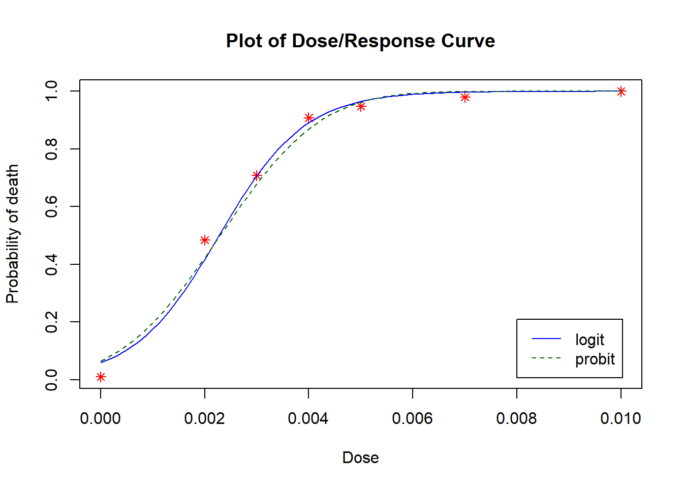
Using this plot, we can decide which model fits the observations best. Both models appear to model the observed probabilities similarly. The logit model appears to model the predicted probabilities more closely to the observed probabilities. As such, we will analyze this model. Recall the model output:
##
## Call:
## glm(formula = response ~ dose, family = binomial(link = "logit"),
##     data = insecticide)
##
## Coefficients:
##              Estimate Std. Error z value Pr(>|z|)
## (Intercept)   -2.7636     0.3006  -9.195   <2e-16 ***
## dose        1215.5565   103.6385  11.729   <2e-16 ***
## ---
## Signif. codes:  0 '***' 0.001 '**' 0.01 '*' 0.05 '.' 0.1 ' ' 1
##
## (Dispersion parameter for binomial family taken to be 1)
##
##     Null deviance: 433.593  on 6  degrees of freedom
## Residual deviance:  13.457  on 5  degrees of freedom
## AIC: 39.287
##
## Number of Fisher Scoring iterations: 5Now, let’s estimate the median lethal dose, \(\delta_{0.5}\). For the logit link, recall that we calculate \(\delta_{0.5}\) as
\[ \delta_{0.5} = \frac{-\beta_0}{\beta_1} \]
which can be estimated by \[ \begin{aligned} \widehat{\delta}_{0.5} &= \frac{-\widehat{\beta}_0}{\widehat{\beta}_1}\\ &=\frac{-(-2.7636)}{1215.5565}\\ &= 0.0023. \end{aligned} \] That is, based on the logit model we estimate the median lethal dose at which 50% of the population will die to be 0.0023.
For more information on dose response models, readers are directed to (Kerr and Meador 1996) and (Karunarathne et al. 2022).
4.8 Poisson Distributed Outcomes (Log-linear Regression)
Data involving counts of events is commonly used in research, and can be analyzed using a Poisson GLM with a log link (also referred to as log-linear regression). That is, we model \[ log(\mu_i) = \boldsymbol{x}_i^T\boldsymbol{\beta}. \] We look at count data in terms of the underlying counting process. We often assume that the counting process can be classified as a Poisson process, meaning:
- The number of events in one interval is independent of the number events in a different interval
- The distribution of the number of events occurring from (0, t] (denoted \(N(t)\)) is given by \[ Pr(N(t) = n; \lambda) = \frac{(\lambda t)^ne^{-\lambda t}}{n!} \] where \(!\) represents the factorial function (for example, \(4! = 4\times 3\times 2 \times 1\)) and \(\lambda\) is a rate parameter. The expected number of events for an interval of length \(t\) is \(E(N(t)) = \mu(t) =\lambda t\). This is a time-homogeneous Poisson process since \(\lambda\) is constant, and is not a function of time.
Under the log link, \[ \begin{aligned} \log(\mu(t)) &= \log(\lambda t)\\ &= \log(\lambda) + \log(t) \end{aligned} \] by the rules of logarithm operations.
If for each subject we observe the number of events from \((0, t_i]\), along with covariates \(x_{i1}, ..., x_{ip}\), then we can model \[ \begin{aligned} \log(\mu_i(t_i)) &= \log(\lambda_i t_i)\\ &= \log(\lambda_i) + \log(t_i)\\ &= \boldsymbol{x_i}^T\boldsymbol{\beta} + \log(t_i). \end{aligned} \] That is, we model our log-linear regression with an offset term of \(\log(t_i)\) that will explain some of the variation in the differing counts of outcomes due to differing lengths of time (or another appropriate measure, depending on the context of the problem). We note that in some cases, an offset term may not be necessary.
4.8.1 Example
Let’s look at an example of a data set that records the number of times an incident occurs in cargo ships (McCullagh and Nelder 2019), which can be found in the MASS package. We can load the data set and look at the first 6 observations using:
##   type year period service incidents
## 1    A   60     60     127         0
## 2    A   60     75      63         0
## 3    A   65     60    1095         3
## 4    A   65     75    1095         4
## 5    A   70     60    1512         6
## 6    A   70     75    3353        18
We have the variable type corresponding to the type of ship (A - E), year which is the year of construction (coded as “60” for 1960-1964, “65” for 1965 - 1969, and so on), period which similarly codes the year of operation (which is either “60” for 1960-1974 or “75” for 1975-1979), service which is the number of months of service for the ship, and incidents which is the number of damage incidents for the ship during the months of service.
We wish to see which factors are associated with ship incidents. To see the distribution of our outcome, we can create a histogram by:
hist(ships$incidents, main = "Histogram of Incidents", ylab = "Frequency",
     xlab = "Number of Incidents")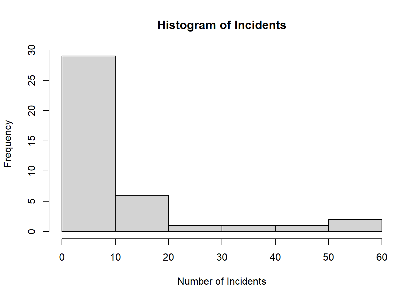
Figure 4.13: Plot showing frequency of incidents for the ships data set. Data is clearly non-normal.
From 4.13, we see that our distribution of the outcome is not symmetric (very skewed to the right), indicating that we cannot use a linear model (which assumes normality of the outcome). This is expected as we are modelling counts of incidents.
In this data set, as different ships will be in service for different months (which may affect how many incidents the ship has), we can use that variable (which is a measure of time) as our offset term. Specifically, we will fit a Poisson regression model using incidents as our outcome and log(service) as the offset term.
We should first clean the data set. This involves changing all of the categorical variables to factors, and removing ships that were never in service:
# create new variables in the data set that are factors
ships$type_f <- as.factor(ships$type)
ships$year_f <- as.factor(ships$year)
ships$period_f <- as.factor(ships$period)

# remove ships (rows) that were never in service (service == 0)
# find which rows have service == 0
toremove <- which(ships$service == 0)

# remove the rows=
ships <- ships[-toremove, ] # the - sign removes the given rows
4.8.1.1 Model Fitting
We start with a main-effects only model using all of the covariates at our disposal. We fit this model in R by
ships_fit1 <- glm(incidents ~ type_f + year_f +period_f +
                   offset(log(service)),
                 family = poisson, data = ships)

# look at the model output
summary(ships_fit1)
##
## Call:
## glm(formula = incidents ~ type_f + year_f + period_f + offset(log(service)),
## family = poisson, data = ships)
##
## Coefficients:
## Estimate Std. Error z value Pr(>|z|)
## (Intercept) -6.40590 0.21744 -29.460 < 2e-16 ***
## type_fB -0.54334 0.17759 -3.060 0.00222 **
## type_fC -0.68740 0.32904 -2.089 0.03670 *
## type_fD -0.07596 0.29058 -0.261 0.79377
## type_fE 0.32558 0.23588 1.380 0.16750
## year_f65 0.69714 0.14964 4.659 3.18e-06 ***
## year_f70 0.81843 0.16977 4.821 1.43e-06 ***
## year_f75 0.45343 0.23317 1.945 0.05182 .
## period_f75 0.38447 0.11827 3.251 0.00115 **
## ---
## Signif. codes: 0 '***' 0.001 '**' 0.01 '*' 0.05 '.' 0.1 ' ' 1
##
## (Dispersion parameter for poisson family taken to be 1)
##
## Null deviance: 146.328 on 33 degrees of freedom
## Residual deviance: 38.695 on 25 degrees of freedom
## AIC: 154.56
##
## Number of Fisher Scoring iterations: 5We should test to see if we can remove any covariates by performing likelihood ratio tests (LRTs) on nested models. We first fit a model without type_f and see if the fit is adequate compared to the main-effects only model. In this setting, we are testing the null hypothesis that the simpler model without type_f is adequate compared to the main-effects only model. If we reject the null, that means that type_f should be included in the model (when we compare it to the main-effects only model). We do this in R as:
# fit the new, nested model
ships_fit2 <- glm(incidents ~ year_f +period_f + # remove type_f as variable
offset(log(service)),
family = poisson, data = ships)
# perform the LRT
anova(ships_fit1, ships_fit2, test = "LRT")## Analysis of Deviance Table
##
## Model 1: incidents ~ type_f + year_f + period_f + offset(log(service))
## Model 2: incidents ~ year_f + period_f + offset(log(service))
## Resid. Df Resid. Dev Df Deviance Pr(>Chi)
## 1 25 38.695
## 2 29 62.365 -4 -23.67 9.3e-05 ***
## ---
## Signif. codes: 0 '***' 0.001 '**' 0.01 '*' 0.05 '.' 0.1 ' ' 1We see from the output we have a small \(p\)-value, indicating that we reject the null hypothesis and conclude that the main-effects only model including type_f is a better fit.
Next we can check if we should remove year_f in a similar manner.
# fit the new, nested model
ships_fit3 <- glm(incidents ~ type_f +period_f + # remove year_f as variable
offset(log(service)),
family = poisson, data = ships)
# perform the LRT
anova(ships_fit1, ships_fit3, test = "LRT")## Analysis of Deviance Table
##
## Model 1: incidents ~ type_f + year_f + period_f + offset(log(service))
## Model 2: incidents ~ type_f + period_f + offset(log(service))
## Resid. Df Resid. Dev Df Deviance Pr(>Chi)
## 1 25 38.695
## 2 28 70.103 -3 -31.408 6.975e-07 ***
## ---
## Signif. codes: 0 '***' 0.001 '**' 0.01 '*' 0.05 '.' 0.1 ' ' 1We again have a small \(p\)-value and reject the null hypothesis that the simpler model fit is adequate. That is, the main-effects only model fits better between these two models.
Next, we test for period_f.
# fit the new, nested model
ships_fit4 <- glm(incidents ~ type_f + year_f + # remove period_f as variable
offset(log(service)),
family = poisson, data = ships)
# perform the LRT
anova(ships_fit1, ships_fit4, test = "LRT")## Analysis of Deviance Table
##
## Model 1: incidents ~ type_f + year_f + period_f + offset(log(service))
## Model 2: incidents ~ type_f + year_f + offset(log(service))
## Resid. Df Resid. Dev Df Deviance Pr(>Chi)
## 1 25 38.695
## 2 26 49.355 -1 -10.66 0.001095 **
## ---
## Signif. codes: 0 '***' 0.001 '**' 0.01 '*' 0.05 '.' 0.1 ' ' 1Again, we have a small \(p\)-value and choose the main-effects only model.
Although we were unable to remove any covariates, we can still test for possible interactions of the covariates. We again perform LRTs where in this setting, the main effects model will be nested in the model that includes additional interactions.
Let’s first start by seeing if we should have an interaction between type_f and year_f. We do this by fitting a new interaction model and comparing it to the main-effects only model. The null hypothesis here is that the main-effects only model (simpler model) fits as well as the interaction model (more complex model). Rejecting the null hypothesis will tell us that we should include the interaction effect in the final model. We do this in R by:
# fit the new interaction model
ships_fit5 <- glm(incidents ~ type_f + year_f + period_f +
type_f*year_f + offset(log(service)), #include interaction
family = poisson, data = ships)
# perform the LRT
anova(ships_fit5, ships_fit1, test = "LRT")## Analysis of Deviance Table
##
## Model 1: incidents ~ type_f + year_f + period_f + type_f * year_f + offset(log(service))
## Model 2: incidents ~ type_f + year_f + period_f + offset(log(service))
## Resid. Df Resid. Dev Df Deviance Pr(>Chi)
## 1 13 14.587
## 2 25 38.695 -12 -24.108 0.01966 *
## ---
## Signif. codes: 0 '***' 0.001 '**' 0.01 '*' 0.05 '.' 0.1 ' ' 1With a small \(p\)-value, we reject the null hypothesis. That is, we conclude the main-effects only (simpler) model is not adequate and we should have this interaction in the final model. Let’s take a look at the model summary here:
##
## Call:
## glm(formula = incidents ~ type_f + year_f + period_f + type_f *
## year_f + offset(log(service)), family = poisson, data = ships)
##
## Coefficients:
## Estimate Std. Error z value Pr(>|z|)
## (Intercept) -23.9891 6625.5246 -0.004 0.99711
## type_fB 17.0506 6625.5246 0.003 0.99795
## type_fC 17.0863 6625.5246 0.003 0.99794
## type_fD -0.5962 9331.1044 0.000 0.99995
## type_fE 0.8799 11522.0953 0.000 0.99994
## year_f65 18.0324 6625.5246 0.003 0.99783
## year_f70 18.3969 6625.5246 0.003 0.99778
## year_f75 18.2860 6625.5246 0.003 0.99780
## period_f75 0.3850 0.1186 3.246 0.00117 **
## type_fB:year_f65 -17.3620 6625.5246 -0.003 0.99791
## type_fC:year_f65 -18.6108 6625.5247 -0.003 0.99776
## type_fD:year_f65 -18.4024 11467.2827 -0.002 0.99872
## type_fE:year_f65 0.4496 11522.0953 0.000 0.99997
## type_fB:year_f70 -17.6110 6625.5246 -0.003 0.99788
## type_fC:year_f70 -17.6160 6625.5246 -0.003 0.99788
## type_fD:year_f70 1.0922 9331.1044 0.000 0.99991
## type_fE:year_f70 -0.8285 11522.0953 0.000 0.99994
## type_fB:year_f75 -17.7124 6625.5246 -0.003 0.99787
## type_fC:year_f75 -17.3813 6625.5247 -0.003 0.99791
## type_fD:year_f75 -0.3254 9331.1044 0.000 0.99997
## type_fE:year_f75 -1.8570 11522.0954 0.000 0.99987
## ---
## Signif. codes: 0 '***' 0.001 '**' 0.01 '*' 0.05 '.' 0.1 ' ' 1
##
## (Dispersion parameter for poisson family taken to be 1)
##
## Null deviance: 146.328 on 33 degrees of freedom
## Residual deviance: 14.587 on 13 degrees of freedom
## AIC: 154.45
##
## Number of Fisher Scoring iterations: 17Looking at the model summary, we notice that only one covariate is significant and we have huge standard errors for most of our covariates in the model. This indicates that we have over-parameterized our model as we have 12 interaction terms here. Looking at the full data set, we see that for ships with type D in the year 1960-1964 or 1965-1969 category, there are no events. This could cause issues with the model fitting. As such, despite what the statistical test told us, we should not continue with this model or use any models that include any interactions between type_f and year_f.
Next we can test if we should also have an interaction between type_f and period_f. We test this model to the main effects model (ships_fit). We do this in R by:
# fit the new interaction model
ships_fit6 <- glm(incidents ~ type_f + year_f + period_f +
type_f*period_f + offset(log(service)), #include interaction
family = poisson, data = ships)
# perform the LRT
anova(ships_fit6, ships_fit1, test = "LRT")## Analysis of Deviance Table
##
## Model 1: incidents ~ type_f + year_f + period_f + type_f * period_f +
## offset(log(service))
## Model 2: incidents ~ type_f + year_f + period_f + offset(log(service))
## Resid. Df Resid. Dev Df Deviance Pr(>Chi)
## 1 21 33.756
## 2 25 38.695 -4 -4.9388 0.2936We have a large \(p\)-value, thus we fail to reject the null hypothesis. That is, we conclude the simpler main-effects only model with no interactions is adequate compared to the model with the interaction and continue model building from there.
Next we can test if we should also have an interaction between year_f and period_f. We test this model to the main effects model again.. We do this in R by:
# fit the new interaction model
ships_fit7 <- glm(incidents ~ type_f + year_f + period_f +
year_f*period_f + offset(log(service)), #include interaction
family = poisson, data = ships)
# perform the LRT
anova(ships_fit7, ships_fit1, test = "LRT")## Analysis of Deviance Table
##
## Model 1: incidents ~ type_f + year_f + period_f + year_f * period_f +
## offset(log(service))
## Model 2: incidents ~ type_f + year_f + period_f + offset(log(service))
## Resid. Df Resid. Dev Df Deviance Pr(>Chi)
## 1 23 36.908
## 2 25 38.695 -2 -1.7875 0.4091We have a large \(p\)-value, thus we fail to reject the null hypothesis. That is, we conclude themain-effects only model is adequate compared to the one with the interaction.
We finish our model building process and conclude that ships_fit1 is the best fitting model of the ones we tested. From the main-effects only model output shown earlier, we see that all covariates have small standard errors, and most levels of the categorical covariates are significant. This is what we should expect from a final model after cycling through the fitting procedure.
4.8.1.2 Model Diagnostics
Residuals
Once we settle on a model from the likelihood ratio tests and initial inspection, we need to check the overall model fit. The first thing we can do is look at a plot of the residual versus fitted values to see if there are any large residuals indicating poor fit in the model. The following code can be used to produce such plots:
resid <- residuals.glm(ships_fit1)
fitted <- ships_fit1$fitted.values
plot(fitted, resid, ylim = c(-3, 3), ylab = "Deviance Residuals", xlab = "Fitted Values")
abline(h = -2, lty = 2)
abline(h = 2, lty = 2)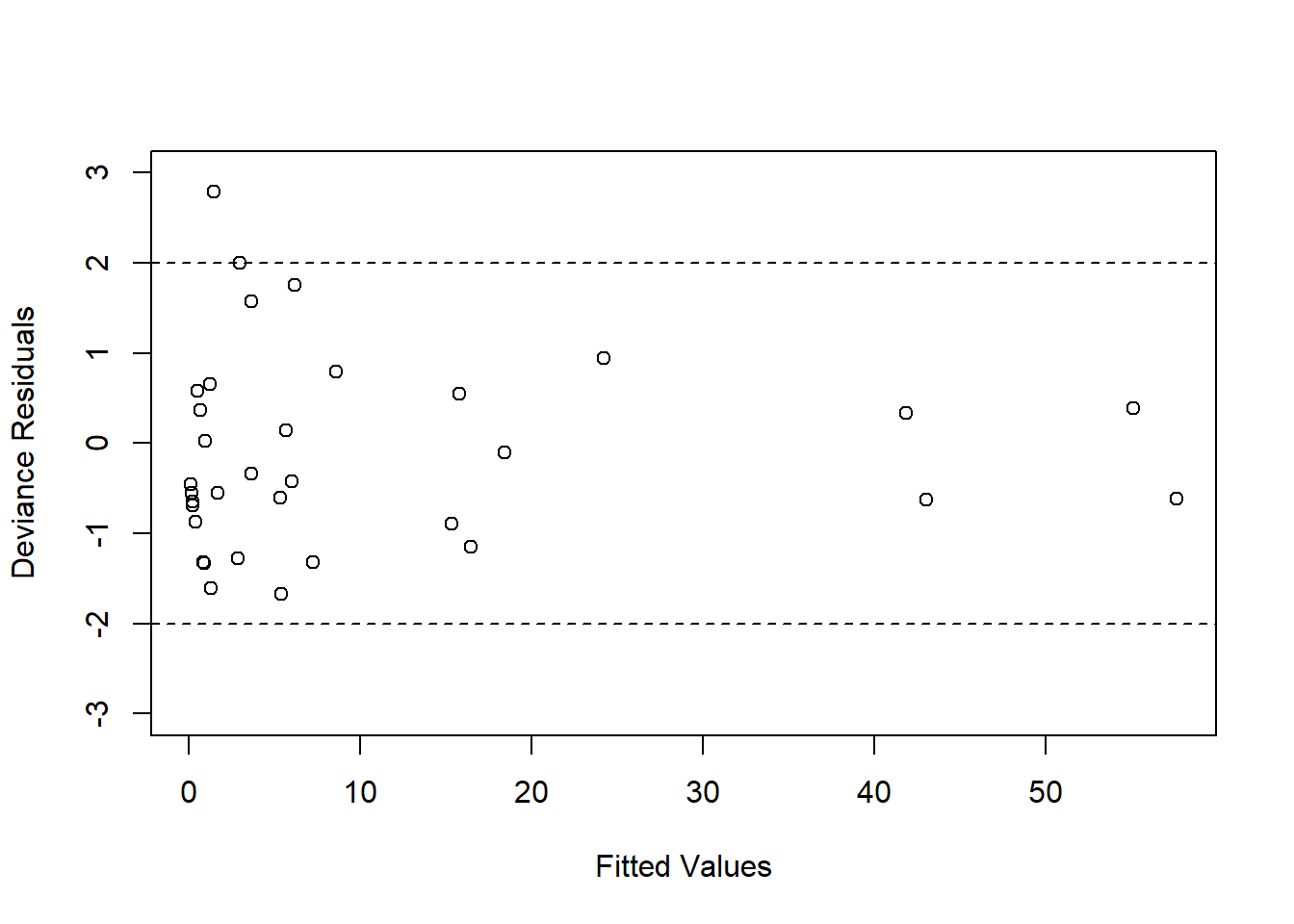
Figure 4.14: Residual diagnostic plot for Poisson GLM.
We see that most values fall within 2 standard deviations, and there do not appear to be extreme residuals.
Overdispersion
A common issue of Poisson GLMs is overdispersion where we have a larger variation in the data set then would expect for the Poisson model (where in this distribution, we have that the mean and variance are equal to each other). When overdispersion occurs, the standard errors of our regression coefficients may be underestimated and we must adjust them. To test for overdispersion, we can use the dispersiontest() function from the AER package. A small \(p\)-value indicates that we reject the null hypothesis that our dispersion is less than one (no overdispersion present). We can perform this test on our model by:
##
## Overdispersion test
##
## data: ships_fit1
## z = 0.9216, p-value = 0.1784
## alternative hypothesis: true dispersion is greater than 1
## sample estimates:
## dispersion
## 1.313931We have a moderately large \(p\)-value of 0.1784, so we fail to reject the null hypothesis. That is, we do not have evidence of overdispersion in this model and continue our analysis.
If overdispersion is present in a model, one can use an ad-hoc approach to estimate a dispersion parameter or use a mixed model (negative binomial distribution) that introduces a random variable that acts as a dispersion factor. For more information on these models, see this tutorial which provides examples in both R and SAS.
Zero-inflation
We should also check if the amount of observed zeros in our outcome marches what would be predicted from our model. If the amount of predicted zeros is smaller than what is observed, we may need to use a zero-inflated poisson regression. We can check for this looking at the ratio of observed versus predicted zeros. This can be done using the check_zeroinflation() function from the performance package in R:
## # Check for zero-inflation
##
## Observed zeros: 8
## Predicted zeros: 8
## Ratio: 1.00## Model seems ok, ratio of observed and predicted zeros is
## within the tolerance range.We see that we have the same number of observed and predicted zeros in the model, and thus we do not need to use a zero-inflated model. There are no strict guidelines for what ratio a zero-inflated model must be used, but it is common for a ratio between 0.95 and 1.05 to be considered good enough to continue with a regular Poisson GLM. More discussion on this issue, along with some more formal statistical tests, can be found here.
Multicollinearity
We should also perform a check on the covariates included in the model.
## GVIF Df GVIF^(1/(2*Df))
## type_f 1.341054 4 1.037363
## year_f 1.524809 3 1.072842
## period_f 1.185194 1 1.088666All VIF values are low, which indicates that there are no issues with multicollinearity in the model.
4.8.1.3 Model Interpretation and Hypothesis Testing
After checking the fit of our model, we can interpret our model to answer the research question of interest. Here, we are interested in seeing if the type of ship, the year it was built, or the period of operation are associated with an increase or decrease in the number of damage incidents.
We can see a summary of the final model again by calling:
##
## Call:
## glm(formula = incidents ~ type_f + year_f + period_f + offset(log(service)),
##     family = poisson, data = ships)
##
## Coefficients:
##             Estimate Std. Error z value Pr(>|z|)
## (Intercept) -6.40590    0.21744 -29.460  < 2e-16 ***
## type_fB     -0.54334    0.17759  -3.060  0.00222 **
## type_fC     -0.68740    0.32904  -2.089  0.03670 *
## type_fD     -0.07596    0.29058  -0.261  0.79377
## type_fE      0.32558    0.23588   1.380  0.16750
## year_f65     0.69714    0.14964   4.659 3.18e-06 ***
## year_f70     0.81843    0.16977   4.821 1.43e-06 ***
## year_f75     0.45343    0.23317   1.945  0.05182 .
## period_f75   0.38447    0.11827   3.251  0.00115 **
## ---
## Signif. codes:  0 '***' 0.001 '**' 0.01 '*' 0.05 '.' 0.1 ' ' 1
##
## (Dispersion parameter for poisson family taken to be 1)
##
##     Null deviance: 146.328  on 33  degrees of freedom
## Residual deviance:  38.695  on 25  degrees of freedom
## AIC: 154.56
##
## Number of Fisher Scoring iterations: 5
We can write this model as \[ \log(\mu(t)) = \beta_0 + \beta_1x_1 + \beta_2x_2 + \beta_3x_3 + \beta_4x_4 + \beta_5x_5 + \beta_6x_5 + \beta_7x_7 + \beta_8x_8 \] where \(x_1\) indicates the ship is type B, \(x_2\) indicates the ship is type C, \(x_3\) indicates the ship is type D, \(x_4\) indicates the ship is type E, \(x_5\) indicates the ship was built between 1965-1969, \(x_6\) indicates the ship was built between 1970-1974, \(x_7\) indicates the ship was built between 1974-1979, \(x_8\) indicates the ship operated between 1975-1979.
Each coefficient can be interpreted as the expected log relative rate (log RR) of incidents. For example, the coefficient for the B type ships (\(\beta_1\) or type_fB from the output) is -0.543 which means that for ships constructed in the same year and that operated in the same period, the rate of incidents for ships of type B is \(\exp(\) -0.543 \()\) = 0.581 times larger than type A ships (the reference group). This indicates that risk of type B ships having incidents was less than that of type A ships (since RR < 1), controlling for period of operation and construction year.
To obtain a confidence interval for this estimate, we can calculate the confidence interval for the log relative rate, and then exponentiate it. In this case, a 95% confidence interval for the log relative rate of incidents for B type ships versus A type ships is \(\widehat{\beta_1} \pm\) 1.960 \(\times \widehat{se}(\widehat{\beta_1})\) = -0.543 \(\pm\) 1.960 \(\times\) 0.178 = (-0.891,-0.195). Then, we take those two numbers and exponentiate them to get a 95% confidence interval for the relative rate, which is (\(\exp(\)-0.891),\(\exp(\)-0.195)) = (0.41,0.823). As this confidence interval does not contain RR = 1, we conclude that the relative rate of incidents for type B ships is significantly lower (since RR < 1) than type A when controlling for period of operation and construction year. Other individual covariates can be similarly interpreted, and confidence intervals for the respective relative rates can easily be found using the confint() function from the MASS package. For example, we can call
## Waiting for profiling to be done...## 2.5 % 97.5 %
## (Intercept) 0.001066843 0.002504456
## type_fB 0.414219640 0.832326237
## type_fC 0.252462723 0.928188620
## type_fD 0.510932360 1.608409891
## type_fE 0.866347032 2.192855450
## year_f65 1.503089957 2.705068073
## year_f70 1.627883790 3.169892062
## year_f75 0.987734160 2.469126537
## period_f75 1.165784432 1.854109971to obtain the 95% individual confidence intervals for the relative rate (after exponentiating). Other confidence intervals can be calculated by changing the level parameter in the confint() function.
If we wanted to compare two ship types to each other where one is not the baseline value in the model, we can still do so with such models. For example, say we want to estimate the relative rate of incidents for ships of type E (\(x_4 = 1\)) versus C (\(x_2 = 1\)), controlling for construction year and period of operation. It is often helpful to create a table such as: \[ \begin{aligned} & \beta_0 + \beta_1x_1 + \beta_2x_2 + \beta_3x_3 + \beta_4x_4 + \beta_5x_5 +\beta_6x_6 + \beta_7x_7 + \beta_8x_8\\ -& (\beta_0 + \beta_1x_1 + \beta_2x_2 + \beta_3x_3 + \beta_4x_4 + \beta_5x_5 +\beta_6x_6 + \beta_7x_7 + \beta_8x_8)\\ & \hline \qquad \qquad \qquad \qquad \qquad \qquad?? \end{aligned} \] and then fill in the values for each scenario. The top row will be for the type E ship and the second row will be for the type C ship. Note that when we fill in 0 for the other types of ships since this is a categorical variable. We also hold the period of operation and construction year constant, so we can just leave these as arbitrary \(x\) values. Then, we perform the subtraction:
\[ \begin{aligned} & \beta_0 + \beta_1(0) + \beta_2(0)+ \beta_3(0) + \beta_4(1) + \beta_5x_5 +\beta_6x_6 + \beta_7x_7 + \beta_8x_8\\ -& (\beta_0 + \beta_1(0) + \beta_2(1) + \beta_3(0) + \beta_4(0) + \beta_5x_5 +\beta_6x_6 + \beta_7x_7 + \beta_8x_8)\\ & \hline \qquad \quad \qquad -\beta_2 \qquad \qquad \quad +\beta_4\\ \end{aligned} \]
So, the log relative rate we wish to calculate is \(-\beta_2 + \beta_4\) = 0.687 + 0.326 = 1.013. To obtain a confidence interval for this quantity, we first need to obtain the estimated standard error of \(-\beta_2 + \beta_4\). We can do this in R by first creating a vector indicating the quantity we’d like to calculate the standard error for (here it is \((\beta_0, \beta_1, \beta_2, \beta_3, \beta_4, \beta_5, \beta_6, \beta_7, \beta_8) = (0, 0, -1, 0 , 1, 0, 0, 0, 0)\)) and then calculating the error by:
# create the vector for -beta2 + beta4 (don't forget to include beta0!)
L <- c(0, 0, -1, 0, 1, 0, 0, 0, 0)

# grab variance-covariance matrix from the model
vcov <- summary(ships_fit1)$cov.unscaled

esterror <- sqrt(t(L) %*% vcov %*% L) #%*% represents matrix multiplication
esterror
## [,1]
## [1,] 0.3394497Then, we can use this in our confidence interval for the log relative rate:
# calculate -beta2 + beta4
estimate <- coef(ships_fit1)%*%L

# calculate lower CI bound
CI_lower <- estimate - 1.96*esterror

# calculate upper CI bound
CI_upper <- estimate + 1.96*esterror

# print it out nicely
print(paste("(", round(CI_lower,3), ",", round(CI_upper,3), ")"))
## [1] "( 0.348 , 1.678 )"Then to get the estimated CI for the relative rate (not log relative rate), we exponentiate both ends of the interval:
# calculate lower CI bound for RR
CI_RR_lower <- exp(CI_lower)

# calculate upper CI bound for RR
CI_RR_upper <- exp(CI_upper)

# print it out nicely
print(paste("(", round(CI_RR_lower,3), ", ", round(CI_RR_upper,3), ")", sep = ""))
## [1] "(1.416, 5.356)"As the resultant confidence interval for the relative rate does not contain an estimate of RR = 1, we conclude that the relative rate of incidents for ships of type E (\(x_4 = 1\)) versus C (\(x_2 = 1\)) significantly differs and is estimated to be 1.013 (95% CI: ), controlling for construction year and period of operation.
For non-categorical variables, the interpretation of the regression coefficient is the log relative rate associated with a one-unit increase in that variable.
For more information on Poisson models, readers are directed to (Hilbe, Zuur, and Ieno 2013), (McCullagh and Nelder 2019).
4.9 Gamma Distributed (Skewed) Outcomes
For continuous data that is not normally distributed, a GLM using the Gamma distribution can be used to model skewed, positive outcomes.
Below are a few examples of Gamma distributions with varying parameters (referred to as the shape and scale parameters).
par(mfrow = c(2,2))
curve(dgamma(x, shape = 1.5, scale = 1), from = 0, to = 10, col = "red",
      main = "Shape = 1.5, Scale = 1",
      xlab = "x",
      ylab = "Density",
      ylim = c(0,1))
curve(dgamma(x, shape = 2.5, scale = 1), from = 0, to = 10, col = "steelblue",
      main = "Shape = 2.5, Scale = 1",
      xlab = "x",
      ylab = "Density",
      ylim = c(0,1))
curve(dgamma(x, shape = 1.5, scale = 0.5), from = 0, to = 10, col = "darkgreen",
      main = "Shape = 1.5, Scale = 0.5",
      xlab = "x",
      ylab = "Density",
      ylim = c(0,1))
curve(dgamma(x, shape = 2.5, scale = 0.5), from = 0, to = 10, col = "purple",
      main = "Shape = 2.5, Scale = 0.5",
      xlab = "x",
      ylab = "Density",
      ylim = c(0,1))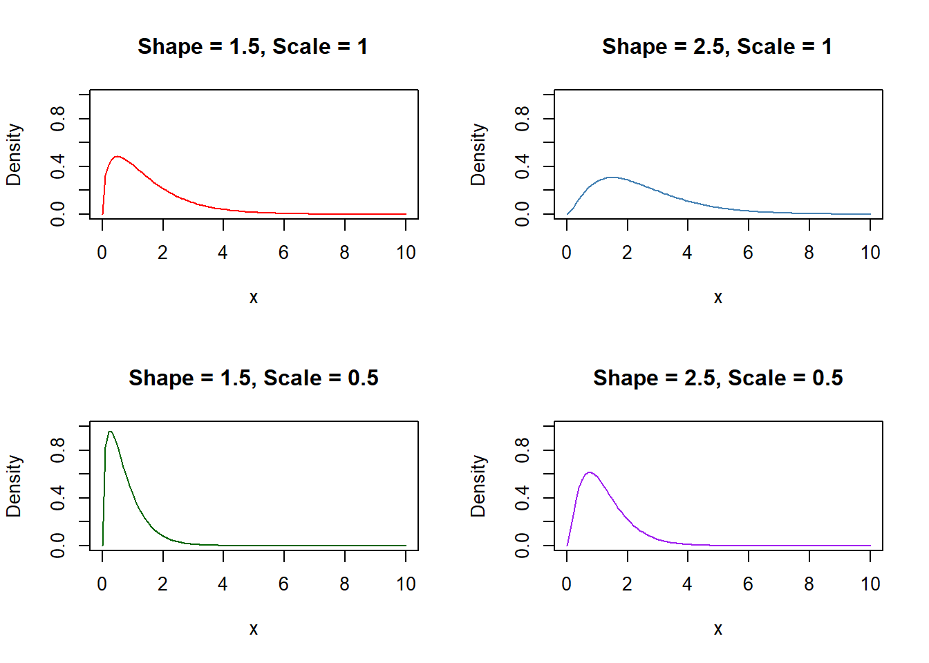
Figure 4.15: Examples of the Gamma distribution. Shape changes across rows while scale changes across columns.
We can see from these four examples that the Gamma distribution is very flexible for modelling continuous outcomes that are skewed and positive. We however note that under the Gamma distribution, the variance is equal to the mean squared, meaning that the ratio of the mean and standard deviation is constant. Using a log link can stabilize the variance, as discussed in (Myers and Montgomery 1997). Although the canonical link for a Gamma family GLM is the inverse link, we commonly see the log link applied in practice because of its interpretations and variance stabilization. Using the log link does not require further constraints on the model when fit.
Under the log link, we model \[ \log(y_{i}) = \boldsymbol{x}_i^T\boldsymbol{\beta} \] which can also be written as \[ \begin{aligned} y_i &= \exp(\boldsymbol{x}_i^T\boldsymbol{\beta})\\ &= \exp(\beta_0 + \beta_1x_{i1} + \beta_2x_{i2} + ... + \beta_{ip}x_{ip})\\ &= \exp(\beta_0)\exp(\beta_1x_{i1}) \exp(\beta_2x_{i2})\dots \exp(\beta_{ip}x_{ip}) \\ &= \exp(\beta_0)\exp(\beta_1)^{x_{i1}} \exp(\beta_2)^{x_{i2}}...\exp(\beta_{ip})^{x_{ip}}. \end{aligned}.\ \] Under the log link, we have a multiplicative model. We interpret \(\exp(\beta_0)\) as the expected value of \(y\) when all covariates are equal to zero. We interpret \(\exp(\beta_j\)) as the expected multiplicative increase of \(y\) for a one unit increase in \(x_j\), when the other covariates are equal to zero. We note that covariates can either be continuous or categorical.
4.9.1 Example
We will re-use the data presented in Section 4.5.1 on rent prices in Munich in 2003. Instead of looking at the clear rent per square meter (rentm) as we did in Section 4.5.1, we will be using the clear rent (without adjustment for apartment area) as the outcome, (rent).
If the data has not already been loaded in from the catdata package, we can load it in and look at first 6 observations using the following code:
##     rent rentm size rooms year area good best warm central tiles
## 1 741.39 10.90   68     2 1918    2    1    0    0       0     0
## 2 715.82 11.01   65     2 1995    2    1    0    0       0     0
## 3 528.25  8.38   63     3 1918    2    1    0    0       0     0
## 4 553.99  8.52   65     3 1983   16    0    0    0       0     0
## 5 698.21  6.98  100     4 1995   16    1    0    0       0     0
## 6 935.65 11.55   81     4 1980   16    0    0    0       0     0
##   bathextra kitchen
## 1         0       0
## 2         0       0
## 3         0       0
## 4         1       0
## 5         1       1
## 6         0       0
Next, we can plot the outcome to see if it is skewed.
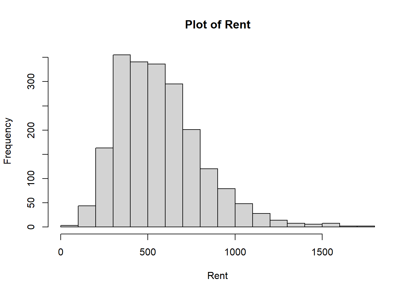
Figure 4.16: Plot used to see if there is any evidence of non-normality in the outcome.
We see that there is some skewness present in the outcome variable. We can confirm this using the Shaprio-Wilk test of normality. Rejecting this test indicates that the normality assumption is not appropriate to use. We can perform this test in R by:
##
##  Shapiro-Wilk normality test
##
## data:  rent$rent
## W = 0.94478, p-value < 2.2e-16
Our \(p\)-value is very small (<0.001) and indicates that we cannot assume the outcome is normal for this data set. As such, we can turn to the Gamma GLM to model this outcome and see if the rent is related to any other covariates in the data set.
4.9.1.1 Model Fitting
We fit a Gamma GLM to the data set with a log link, as described in the previous section. We start by building a main-effects only model containing all possible covariates (aside from rentm). To do so in R, we perform the following:
rent_fit1 <- glm(rent ~ size + factor(rooms) + year + factor(area) +
    factor(good) + factor(best) + factor(warm) + factor(central) +
    factor(tiles) + factor(bathextra) + factor(kitchen), data = rent,
                  family = Gamma(link = "log"))
summary(rent_fit1)
##
## Call:
## glm(formula = rent ~ size + factor(rooms) + year + factor(area) +
## factor(good) + factor(best) + factor(warm) + factor(central) +
## factor(tiles) + factor(bathextra) + factor(kitchen), family = Gamma(link = "log"),
## data = rent)
##
## Coefficients:
## Estimate Std. Error t value Pr(>|t|)
## (Intercept) 0.3241388 0.5371582 0.603 0.546289
## size 0.0118012 0.0004383 26.924 < 2e-16 ***
## factor(rooms)2 0.1004951 0.0208322 4.824 1.51e-06 ***
## factor(rooms)3 0.1101095 0.0260531 4.226 2.48e-05 ***
## factor(rooms)4 0.0383899 0.0353086 1.087 0.277049
## factor(rooms)5 -0.0453271 0.0549179 -0.825 0.409264
## factor(rooms)6 -0.1669296 0.0841069 -1.985 0.047310 *
## year 0.0026328 0.0002727 9.656 < 2e-16 ***
## factor(area)2 -0.0180143 0.0438585 -0.411 0.681310
## factor(area)3 -0.0243536 0.0451711 -0.539 0.589849
## factor(area)4 -0.0580303 0.0446632 -1.299 0.193995
## factor(area)5 -0.0297452 0.0444352 -0.669 0.503313
## factor(area)6 -0.0699323 0.0509111 -1.374 0.169714
## factor(area)7 -0.1591505 0.0507257 -3.137 0.001729 **
## factor(area)8 -0.0717792 0.0517041 -1.388 0.165209
## factor(area)9 -0.0706994 0.0435020 -1.625 0.104277
## factor(area)10 -0.1131664 0.0525807 -2.152 0.031497 *
## factor(area)11 -0.1898598 0.0510428 -3.720 0.000205 ***
## factor(area)12 -0.0526759 0.0484641 -1.087 0.277208
## factor(area)13 -0.0752803 0.0476511 -1.580 0.114304
## factor(area)14 -0.2092354 0.0520687 -4.018 6.07e-05 ***
## factor(area)15 -0.0959255 0.0559367 -1.715 0.086519 .
## factor(area)16 -0.1839807 0.0468027 -3.931 8.75e-05 ***
## factor(area)17 -0.1185536 0.0508523 -2.331 0.019834 *
## factor(area)18 -0.0572051 0.0490754 -1.166 0.243891
## factor(area)19 -0.1330388 0.0470426 -2.828 0.004730 **
## factor(area)20 -0.1082865 0.0534291 -2.027 0.042821 *
## factor(area)21 -0.1364462 0.0521111 -2.618 0.008901 **
## factor(area)22 -0.1961539 0.0659919 -2.972 0.002990 **
## factor(area)23 -0.1694169 0.0791074 -2.142 0.032345 *
## factor(area)24 -0.1685041 0.0623742 -2.702 0.006961 **
## factor(area)25 -0.1635299 0.0464301 -3.522 0.000438 ***
## factor(good)1 0.0600476 0.0143014 4.199 2.80e-05 ***
## factor(best)1 0.1628041 0.0399385 4.076 4.75e-05 ***
## factor(warm)1 -0.3523173 0.0359115 -9.811 < 2e-16 ***
## factor(central)1 -0.1738442 0.0245576 -7.079 2.00e-12 ***
## factor(tiles)1 -0.0816743 0.0146699 -5.567 2.93e-08 ***
## factor(bathextra)1 0.0713144 0.0204249 3.492 0.000491 ***
## factor(kitchen)1 0.1552424 0.0222566 6.975 4.13e-12 ***
## ---
## Signif. codes: 0 '***' 0.001 '**' 0.01 '*' 0.05 '.' 0.1 ' ' 1
##
## (Dispersion parameter for Gamma family taken to be 0.06367392)
##
## Null deviance: 378.02 on 2052 degrees of freedom
## Residual deviance: 143.27 on 2014 degrees of freedom
## AIC: 26142
##
## Number of Fisher Scoring iterations: 5We see many covariates (or levels of a categorical covariate) are statistically significant. We should still, however, see if we can remove some of these covariates to simplify the model. The covariates area has a large number of categories, and some that are not statistically significant. We can investigate whether or not we should include this covariate in the model by fitting a new GLM without area and performing a LRT. We do so with the following code:
# fit the model without factor(area)
rent_fit2 <- glm(rent ~ size + factor(rooms) + year +
factor(good) + factor(best) + factor(warm) + factor(central) +
factor(tiles) + factor(bathextra) + factor(kitchen), data = rent,
family = Gamma(link = "log"))
# perform the LRT
anova(rent_fit2, rent_fit1, test = "LRT")## Analysis of Deviance Table
##
## Model 1: rent ~ size + factor(rooms) + year + factor(good) + factor(best) +
## factor(warm) + factor(central) + factor(tiles) + factor(bathextra) +
## factor(kitchen)
## Model 2: rent ~ size + factor(rooms) + year + factor(area) + factor(good) +
## factor(best) + factor(warm) + factor(central) + factor(tiles) +
## factor(bathextra) + factor(kitchen)
## Resid. Df Resid. Dev Df Deviance Pr(>Chi)
## 1 2038 148.46
## 2 2014 143.27 24 5.1891 3.509e-08 ***
## ---
## Signif. codes: 0 '***' 0.001 '**' 0.01 '*' 0.05 '.' 0.1 ' ' 1The results of this test give us a very small \(p\)-value (<0.001) indicating that we reject the null hypothesis that the simpler model fit is adequate. That is, we should not remove area from the model.
We can further see if other covariates should be removed from the model. Some levels of rooms are insignificant, and so we can fit a model without it and again perform a LRT:
# fit the model without factor(area)
rent_fit3 <- glm(rent ~ size + year + factor(area) +
factor(good) + factor(best) + factor(warm) + factor(central) +
factor(tiles) + factor(bathextra) + factor(kitchen), data = rent,
family = Gamma(link = "log"))
# perform the LRT, comparing to fit1 as fit2 was not adequate
anova(rent_fit3, rent_fit1, test = "LRT")## Analysis of Deviance Table
##
## Model 1: rent ~ size + year + factor(area) + factor(good) + factor(best) +
## factor(warm) + factor(central) + factor(tiles) + factor(bathextra) +
## factor(kitchen)
## Model 2: rent ~ size + factor(rooms) + year + factor(area) + factor(good) +
## factor(best) + factor(warm) + factor(central) + factor(tiles) +
## factor(bathextra) + factor(kitchen)
## Resid. Df Resid. Dev Df Deviance Pr(>Chi)
## 1 2019 147.65
## 2 2014 143.27 5 4.3775 1.867e-13 ***
## ---
## Signif. codes: 0 '***' 0.001 '**' 0.01 '*' 0.05 '.' 0.1 ' ' 1The results of this test also give us a very small \(p\)-value (<0.001) indicating that we reject the null hypothesis that the simpler model fit is adequate. That is, we should not remove rooms from the model.
It does not appear that we should reduce the model further, and we can check this by using the step() function to compare different models by the AIC values:
## Start: AIC=26142.16
## rent ~ size + factor(rooms) + year + factor(area) + factor(good) +
## factor(best) + factor(warm) + factor(central) + factor(tiles) +
## factor(bathextra) + factor(kitchen)
##
## Df Deviance AIC
## <none> 143.27 26142
## - factor(bathextra) 1 144.07 26153
## - factor(best) 1 144.38 26158
## - factor(good) 1 144.41 26158
## - factor(tiles) 1 145.21 26171
## - factor(area) 24 148.46 26176
## - factor(central) 1 146.33 26188
## - factor(kitchen) 1 146.51 26191
## - factor(rooms) 5 147.65 26201
## - factor(warm) 1 149.06 26231
## - year 1 149.44 26237
## - size 1 189.89 26872##
## Call: glm(formula = rent ~ size + factor(rooms) + year + factor(area) +
## factor(good) + factor(best) + factor(warm) + factor(central) +
## factor(tiles) + factor(bathextra) + factor(kitchen), family = Gamma(link = "log"),
## data = rent)
##
## Coefficients:
## (Intercept) size factor(rooms)2
## 0.324139 0.011801 0.100495
## factor(rooms)3 factor(rooms)4 factor(rooms)5
## 0.110109 0.038390 -0.045327
## factor(rooms)6 year factor(area)2
## -0.166930 0.002633 -0.018014
## factor(area)3 factor(area)4 factor(area)5
## -0.024354 -0.058030 -0.029745
## factor(area)6 factor(area)7 factor(area)8
## -0.069932 -0.159150 -0.071779
## factor(area)9 factor(area)10 factor(area)11
## -0.070699 -0.113166 -0.189860
## factor(area)12 factor(area)13 factor(area)14
## -0.052676 -0.075280 -0.209235
## factor(area)15 factor(area)16 factor(area)17
## -0.095925 -0.183981 -0.118554
## factor(area)18 factor(area)19 factor(area)20
## -0.057205 -0.133039 -0.108286
## factor(area)21 factor(area)22 factor(area)23
## -0.136446 -0.196154 -0.169417
## factor(area)24 factor(area)25 factor(good)1
## -0.168504 -0.163530 0.060048
## factor(best)1 factor(warm)1 factor(central)1
## 0.162804 -0.352317 -0.173844
## factor(tiles)1 factor(bathextra)1 factor(kitchen)1
## -0.081674 0.071314 0.155242
##
## Degrees of Freedom: 2052 Total (i.e. Null); 2014 Residual
## Null Deviance: 378
## Residual Deviance: 143.3 AIC: 26140The final model selected by a backwards-selection process also kept all of the main effects in the final model.
We can also consider adding interaction terms. year and size are both statistically significant, and perhaps there is an added increase in rent for units of the same size build in newer years. To see if this is true, we can build a model including the interaction term and again perform an LRT against rent_fit1:
# include interaction between year and size
rent_fit4 <- glm(rent ~ size + factor(rooms) + year + factor(area) +
factor(good) + factor(best) + factor(warm) + factor(central) +
factor(tiles) + factor(bathextra) + factor(kitchen) + year*size, data = rent,
family = Gamma(link = "log"))
# show the output
summary(rent_fit4)##
## Call:
## glm(formula = rent ~ size + factor(rooms) + year + factor(area) +
## factor(good) + factor(best) + factor(warm) + factor(central) +
## factor(tiles) + factor(bathextra) + factor(kitchen) + year *
## size, family = Gamma(link = "log"), data = rent)
##
## Coefficients:
## Estimate Std. Error t value Pr(>|t|)
## (Intercept) 2.920e+00 1.441e+00 2.027 0.042819 *
## size -2.215e-02 1.742e-02 -1.271 0.203717
## factor(rooms)2 9.283e-02 2.122e-02 4.375 1.28e-05 ***
## factor(rooms)3 9.764e-02 2.687e-02 3.634 0.000286 ***
## factor(rooms)4 2.470e-02 3.602e-02 0.686 0.492987
## factor(rooms)5 -5.413e-02 5.507e-02 -0.983 0.325738
## factor(rooms)6 -1.799e-01 8.415e-02 -2.138 0.032649 *
## year 1.306e-03 7.353e-04 1.777 0.075755 .
## factor(area)2 -2.065e-02 4.384e-02 -0.471 0.637705
## factor(area)3 -2.636e-02 4.514e-02 -0.584 0.559262
## factor(area)4 -5.953e-02 4.463e-02 -1.334 0.182404
## factor(area)5 -3.256e-02 4.442e-02 -0.733 0.463664
## factor(area)6 -7.244e-02 5.089e-02 -1.424 0.154732
## factor(area)7 -1.609e-01 5.069e-02 -3.174 0.001524 **
## factor(area)8 -7.575e-02 5.171e-02 -1.465 0.143099
## factor(area)9 -7.440e-02 4.350e-02 -1.711 0.087325 .
## factor(area)10 -1.142e-01 5.253e-02 -2.173 0.029865 *
## factor(area)11 -1.902e-01 5.099e-02 -3.730 0.000197 ***
## factor(area)12 -5.657e-02 4.846e-02 -1.167 0.243241
## factor(area)13 -7.876e-02 4.765e-02 -1.653 0.098486 .
## factor(area)14 -2.109e-01 5.203e-02 -4.054 5.23e-05 ***
## factor(area)15 -9.675e-02 5.588e-02 -1.731 0.083549 .
## factor(area)16 -1.864e-01 4.679e-02 -3.983 7.04e-05 ***
## factor(area)17 -1.251e-01 5.089e-02 -2.458 0.014048 *
## factor(area)18 -6.091e-02 4.907e-02 -1.241 0.214655
## factor(area)19 -1.376e-01 4.708e-02 -2.922 0.003517 **
## factor(area)20 -1.119e-01 5.342e-02 -2.094 0.036356 *
## factor(area)21 -1.399e-01 5.209e-02 -2.685 0.007310 **
## factor(area)22 -2.030e-01 6.602e-02 -3.074 0.002138 **
## factor(area)23 -1.740e-01 7.906e-02 -2.201 0.027874 *
## factor(area)24 -1.730e-01 6.235e-02 -2.774 0.005586 **
## factor(area)25 -1.679e-01 4.645e-02 -3.614 0.000309 ***
## factor(good)1 5.901e-02 1.430e-02 4.128 3.80e-05 ***
## factor(best)1 1.615e-01 3.990e-02 4.048 5.35e-05 ***
## factor(warm)1 -3.484e-01 3.595e-02 -9.691 < 2e-16 ***
## factor(central)1 -1.771e-01 2.459e-02 -7.200 8.46e-13 ***
## factor(tiles)1 -8.190e-02 1.466e-02 -5.588 2.61e-08 ***
## factor(bathextra)1 7.039e-02 2.041e-02 3.448 0.000576 ***
## factor(kitchen)1 1.551e-01 2.223e-02 6.977 4.07e-12 ***
## size:year 1.746e-05 8.956e-06 1.949 0.051421 .
## ---
## Signif. codes: 0 '***' 0.001 '**' 0.01 '*' 0.05 '.' 0.1 ' ' 1
##
## (Dispersion parameter for Gamma family taken to be 0.06354123)
##
## Null deviance: 378.02 on 2052 degrees of freedom
## Residual deviance: 143.03 on 2013 degrees of freedom
## AIC: 26141
##
## Number of Fisher Scoring iterations: 5## Analysis of Deviance Table
##
## Model 1: rent ~ size + factor(rooms) + year + factor(area) + factor(good) +
## factor(best) + factor(warm) + factor(central) + factor(tiles) +
## factor(bathextra) + factor(kitchen)
## Model 2: rent ~ size + factor(rooms) + year + factor(area) + factor(good) +
## factor(best) + factor(warm) + factor(central) + factor(tiles) +
## factor(bathextra) + factor(kitchen) + year * size
## Resid. Df Resid. Dev Df Deviance Pr(>Chi)
## 1 2014 143.27
## 2 2013 143.03 1 0.23906 0.05242 .
## ---
## Signif. codes: 0 '***' 0.001 '**' 0.01 '*' 0.05 '.' 0.1 ' ' 1We see that the \(p\)-value of this test is 0.0542. While it is common to only reject null hypotheses when \(p\) < 0.05, many statisticians argue that such cut-offs are arbitrary and should not be used. However, although borderline “statistically significant” according to the common threshold of 0.05, the coefficient on the size:year is very close to zero, indicating no practical significance. As such, we leave it out of the model and continue analysis with rent_fit1.
We note that while other interaction terms can be included, interactions between categorical covariates with a large number of levels may cause issues with the model fitting when sample sizes are small.
4.9.2 Model Diagnostics
We need to evaluate the model fit prior to interpreting the coefficients and determining associations. We begin by looking at the residuals for any outliers, extreme values, or overall poor model fit:
resid_rent <- residuals.glm(rent_fit1)
fitted_rent <- rent_fit1$fitted.values
plot(fitted_rent, resid_rent, ylim = c(-3, 3), ylab = "Deviance Residuals", xlab = "Fitted Values")
abline(h = -2, lty = 2)
abline(h = 2, lty = 2)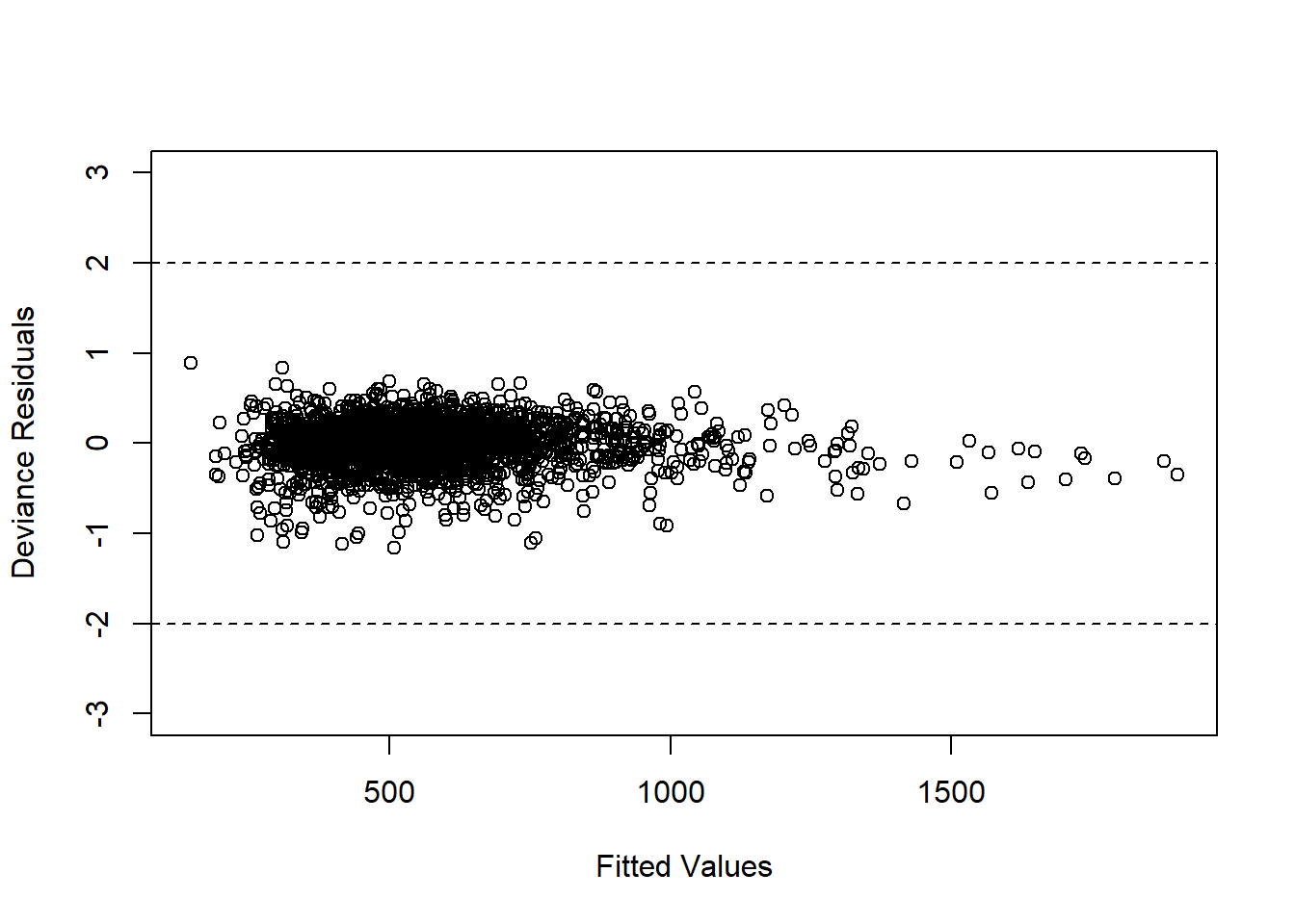
Figure 4.17: Diagnostic plot for Gamma GLM fit
We see that all of the residuals fall between \((-2,2)\), which does not provide any evidence of poor model fit.
We should also check for multicollinearity using the vif() function from the car package:
## GVIF Df GVIF^(1/(2*Df))
## size 3.920003 1 1.979900
## factor(rooms) 3.991510 5 1.148454
## year 1.482946 1 1.217763
## factor(area) 2.528454 24 1.019513
## factor(good) 1.570486 1 1.253190
## factor(best) 1.102579 1 1.050038
## factor(warm) 1.407129 1 1.186225
## factor(central) 1.516196 1 1.231339
## factor(tiles) 1.046607 1 1.023038
## factor(bathextra) 1.134967 1 1.065348
## factor(kitchen) 1.081678 1 1.040037All VIF values are below 10, and as such we do not have reason to be concerned about multicollinearity in this model.
4.9.2.1 Model Interpretation
Recall the final model chosen by the model selection procedure above:
##
## Call:
## glm(formula = rent ~ size + factor(rooms) + year + factor(area) +
##     factor(good) + factor(best) + factor(warm) + factor(central) +
##     factor(tiles) + factor(bathextra) + factor(kitchen), family = Gamma(link = "log"),
##     data = rent)
##
## Coefficients:
##                      Estimate Std. Error t value Pr(>|t|)
## (Intercept)         0.3241388  0.5371582   0.603 0.546289
## size                0.0118012  0.0004383  26.924  < 2e-16 ***
## factor(rooms)2      0.1004951  0.0208322   4.824 1.51e-06 ***
## factor(rooms)3      0.1101095  0.0260531   4.226 2.48e-05 ***
## factor(rooms)4      0.0383899  0.0353086   1.087 0.277049
## factor(rooms)5     -0.0453271  0.0549179  -0.825 0.409264
## factor(rooms)6     -0.1669296  0.0841069  -1.985 0.047310 *
## year                0.0026328  0.0002727   9.656  < 2e-16 ***
## factor(area)2      -0.0180143  0.0438585  -0.411 0.681310
## factor(area)3      -0.0243536  0.0451711  -0.539 0.589849
## factor(area)4      -0.0580303  0.0446632  -1.299 0.193995
## factor(area)5      -0.0297452  0.0444352  -0.669 0.503313
## factor(area)6      -0.0699323  0.0509111  -1.374 0.169714
## factor(area)7      -0.1591505  0.0507257  -3.137 0.001729 **
## factor(area)8      -0.0717792  0.0517041  -1.388 0.165209
## factor(area)9      -0.0706994  0.0435020  -1.625 0.104277
## factor(area)10     -0.1131664  0.0525807  -2.152 0.031497 *
## factor(area)11     -0.1898598  0.0510428  -3.720 0.000205 ***
## factor(area)12     -0.0526759  0.0484641  -1.087 0.277208
## factor(area)13     -0.0752803  0.0476511  -1.580 0.114304
## factor(area)14     -0.2092354  0.0520687  -4.018 6.07e-05 ***
## factor(area)15     -0.0959255  0.0559367  -1.715 0.086519 .
## factor(area)16     -0.1839807  0.0468027  -3.931 8.75e-05 ***
## factor(area)17     -0.1185536  0.0508523  -2.331 0.019834 *
## factor(area)18     -0.0572051  0.0490754  -1.166 0.243891
## factor(area)19     -0.1330388  0.0470426  -2.828 0.004730 **
## factor(area)20     -0.1082865  0.0534291  -2.027 0.042821 *
## factor(area)21     -0.1364462  0.0521111  -2.618 0.008901 **
## factor(area)22     -0.1961539  0.0659919  -2.972 0.002990 **
## factor(area)23     -0.1694169  0.0791074  -2.142 0.032345 *
## factor(area)24     -0.1685041  0.0623742  -2.702 0.006961 **
## factor(area)25     -0.1635299  0.0464301  -3.522 0.000438 ***
## factor(good)1       0.0600476  0.0143014   4.199 2.80e-05 ***
## factor(best)1       0.1628041  0.0399385   4.076 4.75e-05 ***
## factor(warm)1      -0.3523173  0.0359115  -9.811  < 2e-16 ***
## factor(central)1   -0.1738442  0.0245576  -7.079 2.00e-12 ***
## factor(tiles)1     -0.0816743  0.0146699  -5.567 2.93e-08 ***
## factor(bathextra)1  0.0713144  0.0204249   3.492 0.000491 ***
## factor(kitchen)1    0.1552424  0.0222566   6.975 4.13e-12 ***
## ---
## Signif. codes:  0 '***' 0.001 '**' 0.01 '*' 0.05 '.' 0.1 ' ' 1
##
## (Dispersion parameter for Gamma family taken to be 0.06367392)
##
##     Null deviance: 378.02  on 2052  degrees of freedom
## Residual deviance: 143.27  on 2014  degrees of freedom
## AIC: 26142
##
## Number of Fisher Scoring iterations: 5
We can write the chosen model (rent_fit1)) as
\[
\log(y_i) = \beta_0 + \beta_1x_1 + \beta_2x_2 + \beta_3x_3 + \dots + \beta_{38}x_{38}
\]
or equivalently
\[
\begin{aligned}
y_i &= \exp( \beta_0 + \beta_1x_1 + \beta_2x_2 + \beta_3x_3 + \dots + \beta_{38}x_{38})\\
&=\exp(\beta_0)\exp(\beta_1)^{x_1}\exp(\beta_2)^{x_2}\exp(\beta_3)^{x_3}\dots\exp(\beta_{38})^{x_{38}}
\end{aligned}
\]
where \(x_{1}, x_{2}, \dots, x_{38}\) represent each covariate (or level or each covariates) as in the summary of rent_fit1.
From this model, we interpret \(\exp(\beta_0) = \exp(0.324) = 1.383\) as the expected clear rent when all other covariates are 0. For the other covariates, we interpret \(\exp(\beta_j)\) as the expected multiplicative increase of the clear rent for a one unit increase in \(x_j\) when all other covariates are 0. For example, we would interpret \(\exp(\beta_1) = \exp(0.012) = 1.012\) as the expected multiplicative increase of the clear rent for a one unit increase in the living space per squared meter when all other covariates are 0. This result is statistically significant.
We can also use these models to predict. Fore example, if we wanted to predict the clear rent for a 100 square meter home with 2 rooms built in 1995 in municipality 3 with a “good” address, warm water, central heating, no bathroom tiles, no special furniture in the bathroom, and an upmarket kitchen. We can create a new observation as if it is in the data frame and use the predict() function to obtain a prediction. We do this in R by:
# create a data frame using info we want to use to predict
newdata = data.frame(size = 100, rooms = 2, year = 1995,
                     area = 3, good = 1, best = 0, warm = 1,
                     central = 1, tiles = 0, bathextra = 0, kitchen = 1)

#use model to predict value of am
predict(rent_fit1, newdata, type = "response")
## 1
## 679.8872We estimate the clear rent for the above unit to be 679.89 Euros based on the Gamma GLM.
4.10 Further Reading
For a more detailed, theoretical introduction to generalized linear models, readers are directed to (McCullagh and Nelder 2019).