8 Introduction to Sample Size Determination
Author: Luke Hagar
Last Updated: October 17, 2022
8.1 Introduction
Sample size determination involves choosing the number of observations to include in a statistical sample. It is an important component of experimental design. Researchers often visit the SSCR Statistics Help Desk for statistical advice after the data collection process is complete. Sometimes, these researchers have collected very small samples for their study, which can greatly complicate the analysis. In some cases, we may find major flaws in the study design and recommend that they redo the study. To avoid these situations, it is best to thoroughly consider sample size determination while designing a study. We understand that resources such as time and funding are limited, but considering sample size determination beforehand can help (i) set realistic expectations for the study or (ii) support the use of simpler statistical models when analyzing the data.
There are both practical and statistical considerations that inform sample size determination. Practical considerations for sample size determination include the cost of sampling each observation (sometimes called an experimental unit), the time associated with collecting each observation, and the convenience with which observations can be sampled. Statistical considerations include the statistical power (to be discussed) of the designed study and the precision of its relevant estimates. This chapter focuses on the statistical considerations for sample size determination, but it may be useful to also take into account practical considerations when designing the study.
8.1.1 List of R Packages Used
In this chapter, we will be using the packages pwr, TOSTER, foreach, doParallel, and doSNOW. We will also discuss the free sample size determination software G\(^*\)Power.
## Warning: package 'pwr' was built under R version 4.3.3## Warning: package 'TOSTER' was built under R version 4.3.3## Warning: package 'foreach' was built under R version 4.3.3## Warning: package 'doParallel' was built under R version 4.3.3## Warning: package 'iterators' was built under R version 4.3.3## Warning: package 'doSNOW' was built under R version 4.3.3## Warning: package 'snow' was built under R version 4.3.28.1.2 Type I and Type II Errors
Most statistical studies involve testing a hypothesis of interest. When testing a hypothesis using statistical hypothesis tests, we can make two types of errors. To introduce these types of errors, we use a standard two-sample hypothesis test where we wish to test a one-sided hypothesis. We let \(\mu_1\) be the mean response for the first group and \(\mu_2\) be the mean response for the second group. The null and alternative hypotheses for this test are \[H_0: \mu_1 \ge \mu_2 ~~~\text{vs.}~~~ H_A: \mu_1 < \mu_2.\]
We typically decide whether or not to reject the null hypothesis using \(p\)-values. If the \(p\)-value is smaller than a predetermined threshold \(\alpha\), then we reject \(H_0\); otherwise, we do not reject the null hypothesis. This type of standard hypothesis test does not allow us to accept the null hypothesis. In the frequentist framework, we consider \(\mu_1\) and \(\mu_2\) to be fixed, unknown values. Therefore, we do not known whether the statement \(\mu_1 \ge \mu_2\) is true or false, but it is either true or false.
A type I error occurs when we incorrectly reject the null hypothesis. For this example, that means that we reject \(H_0\) when \(\mu_1\) is indeed at least equal to \(\mu_2\). A type II error occurs when we incorrectly do not reject the null hypothesis. For this example, this means that we do not reject \(H_0\) when \(\mu_1\) is less than \(\mu_2\). Before discussing how to control the probability of making a type I or II error, it may be helpful to explain to the researcher what the consequences of making type I and II errors mean in the context of their experiment. Let’s imagine that \(\mu_1\) and \(\mu_2\) represent the mean patient survival time for two types of cancer treatments. Treatment 1 (corresponding to \(\mu_1\)) is the standard existing treatment, whereas treatment 2 (corresponding to \(\mu_2\)) is a novel treatment. Clinicians might recommend replacing the standard treatment with treatment 2 if we obtain enough evidence to reject the null hypothesis \(H_0: \mu_1 \ge \mu_2\). In this situation, a type I error would result in replacing the existing cancer treatment with an inferior one. A type II error would result in not replacing the existing cancer treatment with a superior one. The severity of the consequences associated with making type I and II errors should inform the probability with which researchers are comfortable making them.
We typically control the probability of making a type I error by choosing a significance level \(\alpha\) for the hypothesis test. We reject \(H_0\) if the corresponding \(p\)-value is less than \(\alpha\). For a point null hypothesis (e.g. \(H_0: \mu = 0\)), the \(p\)-value takes values of less than \(\alpha\) with probability \(\alpha\) when \(H_0\) is true. Therefore, the significance level \(\alpha\) is equal to the probability of making a type I error. Controlling the probability of making a type I error is slightly more complicated when the null hypothesis is not a point null hypothesis (e.g. \(H_0: \mu \ge 0\)); in this case, there is more than one value for \(\mu\) such that the null hypothesis would be true. In these situations, the significance level \(\alpha\) determines the size of the hypothesis test. For \(H_0: \mu \ge 0\), let \(\Omega_0 = \{\mu : H_0 ~\text{is true} \}\). The size of the test is then
\[\text{sup}_{\mu^* \in \Omega_0}~Pr( H_0 ~\text{is rejected} ~| ~\mu^* ~\text{is the true parameter value}).\]
Thus, the size of the test is the maximum probability of making a type I error over the entire null hypothesis space \(\Omega_0\). If we use a significance level of \(\alpha\) for the \(p\)-value when conducting a hypothesis test, the size of the test is typically also equal to \(\alpha\). In many situations, the size of the test is equal to the probability of making a type I error at some boundary point of \(\Omega_0\). For this example, that means that our probability of making a type I error might be much lower than the size of the test for certain true \(\mu\) values. For instance, the probability of making a type I error may be equal to \(\alpha\) on the boundary \(\mu = 0\), but it may be much less than \(\alpha\) if the true, unknown value for \(\mu\) is such that \(\mu >> 0\).
We typically control the probability of making a type II error when choosing the sample size for the study. We often let \(\beta\) be the probability of making a type II error and define the power of a hypothesis test as 1 - \(\beta\). Ideally, we want the power of a hypothesis test to be high. In general, the power of a hypothesis test can be made larger by increasing the sample size. The power of a test depends on the size of the effect that we would like to be able to detect. Effect size is discussed in more detail in Section 8.1.3. The effect size can generally been seen as the magnitude of the departure from the null hypothesis. Let’s reconsider the null hypothesis \(H_0: \mu_1 \ge \mu_2\). If \(\mu_2 = \mu_1 + \epsilon\) for some small \(\epsilon > 0\), then we may require a lot of data gather enough evidence to reject the null hypothesis. However, if \(\mu_2 >> \mu_1\), we may not require much data to reject the null hypothesis. As such, effect size is an important consideration for sample size determination.
8.1.3 Effect Size
Generally, the effect size can be seen as the magnitude of the departure from the null hypothesis. It follows that larger departures (effect sizes) should be easier to detect (i.e., we can detect them using smaller samples). We often assume that the data are approximately normal (an appropriate transformation may need to be applied). In this case, we can assume that the observed data \(y_1,...,y_n\) are such that \(Y_i \sim N(\mu, \sigma^2)\) for \(i=1,...,n\) independently. It is often of interest to test the null hypothesis \(H_0: \mu = \mu_0\). For this hypothesis test, the effect size would typically be given by \[d = \frac{\mu - \mu_0}{\sigma}.\] We discuss this further in Section 8.2, but we often need to guess the value of \(\sigma\) to conduct the sample size calculation. For a two-sided hypothesis test, the effect size \(d\) can be positive or negative. Therefore, if the unknown, true value of \(\mu\) is much larger or smaller than \(\mu_0\), we should have greater probability of rejecting the null hypothesis for smaller samples. If we would instead like to conduct a one-sided hypothesis test, we need to more carefully consider the sign of the effect. For instance, we may want to test the null hypothesis \(H_0: \mu \le \mu_0\). In this scenario, it is not seen as a departure from the null hypothesis when \(\mu << \mu_0\). Therefore, we should only consider effect sizes \(d > 0\) when selecting a sample size for the study.
The effect size may also be referred to as Cohen’s \(d\) (Cohen 2013), particularly in scenarios where we want to compare two means using their standardized difference. In these scenarios, our null hypothesis of interest is typically \(H_0: \mu_1 = \mu_2\), and the corresponding effect size is \[d = \frac{\mu_1 - \mu_2}{\sigma}.\]
For the purposes of sample size determination, it is often assumed that the variances for the two normal populations are unknown but the same for both groups. That is, we assume that \(Y_{1j} \sim N(\mu_1, \sigma^2)\) for \(j = 1,...,n_1\) and \(Y_{2j} \sim N(\mu_2, \sigma^2)\) for \(j = 1,...,n_2\). This assumption is typically made for two reasons. First, it simplifies the sample size calculation; we can sometimes compute the sample size that will achieve the desired power for the study using an analytical formula if we assume the variances are the same. We might need to resort to simulation-based sample size determination (discussed in Section 8.3) if we do not make this assumption. Second, it is often difficult enough for the researcher to estimate one value for \(\sigma\). They may not have sufficient information to specify \(\sigma_1\) and \(\sigma_2\), different measures of variability for each group. If the researcher does have sufficient information to estimate \(\sigma_1\) and \(\sigma_2\), the pooled standard deviation could be used for sample size calculations: \[\sigma = \sqrt{\frac{\sigma_1^2}{n_1} + \frac{\sigma_2^2}{n_2}}.\]
Although most researchers visiting the SCCR may not have sufficient funding to obtain extremely large samples, it is important to note that we are able to detect very small effects when the sample size for the study is very large. As such, it is important to justify that the observed effect sizes are practically – and not just statistically – significant. For instance, we may want to test whether the average final grade in STAT 230 is the same as the average final grade in STAT 231. After collecting (potentially hundreds of) observations from each class, we may estimate the average final grades in STAT 230 and STAT 231 to be 75.1% and 75.3%, respectively. We may have collected enough data to conclude that the difference between the average final grades in the two classes is not exactly 0, but an increase of 0.2% might not be very meaningful. Perhaps a 1% difference in the average final grades is the smallest difference that would be practically important – then this knowledge from the researcher should inform the effect size used in the sample size calculation. Researchers should be prepared to justify that their observed effect sizes are meaningful in the context of their discipline. Simply observing a \(p\)-value that is less than the significance level \(\alpha\) may be not be enough to guarantee publication. In recent years, certain journals (e.g. Basic and Applied Psychology and Political Analysis) have actually banned the use of \(p\)-values in their journals as a result of \(p\)-values being misused in certain situations (Wasserstein and Lazar 2016). Certain journals are now placing more emphasis on precise effect estimation over \(p\)-values, which will be discussed briefly in Section 8.1.5. If applicable, it might be helpful for researchers to consider the desired avenue for publication before designing their study.
8.1.4 Equivalence Testing
For certain analyses, researchers may want to collect enough data to show that there is no substantial effect. In certain fields, researchers may try to do this by computing the post-hoc power of a study. For instance, if we did not reject the null hypothesis, we might try to use the observed standard deviation (not the value for \(\sigma\) estimated prior to conducting the study) to determine what our “post-hoc” power is to detect effects of given sizes. This is not the recommended method for concluding that there is no substantial effect; however, certain journal editors or reviewers may request that a post-hoc power analysis be performed. Equivalence testing (Walker and Nowacki 2011) provides a more statistically sound method to conclude that there is no substantial effect. Equivalence testing requires its own sample size determination procedures.
Equivalence testing aims to conclude that the true effect size lies in the interval \((-\delta, \delta)\) for some \(\delta > 0\); this value for \(\delta\) is often referred to as the equivalence margin. For instance, a standard hypothesis test may involve the null hypothesis \(H_0: \mu_1 = \mu_2\). Equivalence testing may instead consider the null hypothesis to be \(H_0: \{\mu_1 - \mu_2 \le -\delta\}\cup\{\mu_1 - \mu_2 \ge \delta\}\). If we reject this hypothesis, we can conclude that \(\mu_1 - \mu_2 \in (-\delta, \delta)\). The value of \(\delta\) should typically be chosen by the researcher – based on what would constitute a substantial effect size in the context of their comparison.
Equivalence testing is often carried out using a two one-sided test (TOST) procedure. For the previous example, we would first test the one-sided null hypothesis \(H_{01}: \mu_1 - \mu_2 \le -\delta\) and then test the second one-sided null hypothesis \(H_{01}: \mu_1 - \mu_2 \ge \delta\). Let’s again assume that \(Y_{1j} \sim N(\mu_1, \sigma^2)\) for \(j = 1,...,n_1\) and \(Y_{2j} \sim N(\mu_2, \sigma^2)\) for \(j = 1,...,n_2\). If we reject both null hypotheses using one-sided \(t\)-tests with significance level \(\alpha\), then we can reject the composite null hypothesis \(H_0: \{\mu_1 - \mu_2 \le -\delta\}\cup\{\mu_1 - \mu_2 \ge \delta\}\) with significance level \(\alpha\) as well. When conducting sample size determination for equivalence tests, we must specify (i) the estimates for quantities from the previous subsection (\(d\), \(\sigma\), etc.) and (ii) the equivalence margin \(\delta\). Cohen (2013) provides some rough context for the standardized effect size \(d\); \(d = 0.2\), \(d = 0.5\), and \(d = 0.8\) respectively correspond to small, medium, and large effect sizes. The equivalence margin \(\delta\) could be chosen to coincide with Cohen’s advice in the absence of strong subject matter expertise. However, subject matter expertise from the researcher should be used to choose \(\delta\) whenever possible. We often require larger sample sizes to achieve the desired power as the equivalence margin \(\delta\) increases to 0.
8.1.5 Precision-Based Sample Size Determination
Researchers may be planning a study where the objective is not to show the absence or presence of an effect. Instead, they might wish to precisely estimate the size of an effect. A researcher may have this objective if alternatives to \(p\)-values are preferred in their field. They may also be conducting a follow-up study: previous work may be concluded that a non-null effect does exist, and they hope to estimate this effect with greater precision than the original study. In these situations, the sample size may be chosen to bound the length of a confidence interval for the true effect size. The most standard formula for an (approximate) confidence interval is \[\hat d \pm z_{1 - \alpha/2}\times s_d/\sqrt{n},\] where \(\hat d\) is the estimate for the effect size \(d\) obtained from the data, \(z_{1 - \alpha/2}\) is the \(1 - \alpha/2\) quantile of the standard normal distribution, and \(s_d\) is the estimated standard deviation of the effect size. In certain situations, it may be more appropriate to use a \(t\)-distribution with \(\nu\) degrees of freedom instead of a normal distribution, or we may wish to consider a non-symmetric confidence interval. In this subsection, we focus only on the case for the simplest formula given above. In this case, the length of the confidence interval is \[2\times z_{1 - \alpha/2}\times s_d/\sqrt{n}.\]
To conduct this sample size determination calculation, we must choose a value \(\alpha\) such that the confidence interval has the desired coverage \(1 - \alpha\). We must also estimate \(\sigma\), the value for \(s_d\) to be used for the purposes of sample size determination. Given \(\alpha\) and \(\sigma\), the length of the confidence interval is a univariate function of \(n\). Given a target length for the confidence interval \(l\), we can choose the sample size to be \[n = \frac{4 \times z_{1 - \alpha/2}^2 \times \sigma^2}{l^2}.\]
We note that the sample sizes returned by this approach may be substantially greater than those returned by the more standard sample size calculations to control type I error and power. For instance, if the true value of the effect is \(d = 10\), we may need much less data to conclude that \(d \ne 0\) than we would need to precisely estimate the effect. The sample size \(n\) is a not a linear function of the target length \(l\). That is, to decrease the length of the confidence interval by a factor of 10, we need to increase the sample size by a factor of \(10^2 = 100\). However, these large sample sizes may be required if we want to estimate effects from the study with the desired level of precision.
8.2 Sample Size Determination for Common Models
8.2.1 The pwr Package
In this subsection, we provide a brief overview of the pwr package and its capabilities. The pwr package contains several types of functions. The first set of functions involve computing effect sizes for common analyses: cohen.ES(), ES.h(), ES.w1(), and ES.w2(). We will discuss the cohen.ES() function in more detail. This function returns the conventional effect sizes (small, medium, and large) for the tests available in the pwr package. This function has two parameters:
testdenotes the statistical test of interest.test = "p"is used for a hypothesis test to compare proportions.test = "t"is used to denote a \(t\)-test to compare means (one-sample, two-sample, or paired samples).test = "r"is used for a hypothesis test to compare correlations.test = "anov"is used to denote balanced one-way analysis of variance (ANOVA) tests.test = "chisq"is used to denote \(\chi^2\) tests for goodness of fit or association between variables. Lastly,test = "f2"is used for a hypothesis test that considers the \(R^2\) statistic from a general linear model.sizedenotes the effect size. It takes one of three values:"small","medium", or"large".
This function is helpful because you do not need to memorize the conventional effect sizes for the common statistical analyses listed above. The following R code shows what this function outputs for a medium effect corresponding to a balanced one-way ANOVA test.
##
##      Conventional effect size from Cohen (1982)
##
##            test = anov
##            size = medium
##     effect.size = 0.25
The effect size itself can be returned directly using the following code. This effect size can be used as an input value for many of the other functions in the pwr package.
## [1] 0.25The remaining functions in the pwr package facilitate power analysis for common statistical analyses: pwr.2p.test(), pwr.2p2n.test(), pwr.anova.test(), pwr.chisq.test(), pwr.f2.test(), pwr.norm.test(), pwr.norm.test(), pwr.p.test(), pwr.r.test(), pwr.t.test(), and pwr.t2n.test(). The functions with 2n in their names allow for power analysis will unequal sample sizes; the other functions force the sample sizes to be the same in each group. We will discuss some of these functions in greater detail later in this section (after introducing G\(^*\)Power). We note that power curves can be plotted for many of these analyses using the standard plot() function. This will also be discussed later in this section.
8.2.2 G*Power Software
G\(^*\)Power is a free sample size determination software developed by Heinrich Heine University Düsseldorf in Germany. G\(^*\)Power is more comprehensive than the pwr package in R. Moreover, the G\(^*\)Power user manual is more detailed than the documentation for the pwr package in R. Although neither G\(^*\)Power nor the pwr package offer complete functionality for sample size determination, they offer a good starting point for common statistical analyses. The interface for G\(^*\)Power might be easier for researchers to use, particularly those who do not have much experience with R. However, if the researcher is already familiar with with R and their desired analysis is supported by the pwr package, then the pwr pacakge may be the more suitable choice.
G\(^*\)Power supports statistical power analyses for many different statistical tests of the \(F\)-test family, the \(t\)-test family, \(\chi^2\)-test family, \(z\)-test family, and even some exact and nonparametric tests. G\(^*\)Power provides both effect size calculators and graphics options. G\(^*\)Power offers five different types of statistical power analysis. First, it supports a priori analysis, where the sample size \(N\) is computed as a function of power level \(1 - \beta\), significance level \(\alpha\), and the to-be-detected population effect size. This is the most common type of power analysis. Second, it supports compromise power analysis, where both \(1 - \alpha\) and \(\beta\) are computed as functions of the effect size, \(N\), and an error probability ratio \(q = \beta/\alpha\). Third, it supports criterion power analysis, where the significance level \(\alpha\) is chosen to obtain the desired power \(1 - \beta\) for a given effect size and \(N\). Fourth, it supports post-hoc poweranalysis, where \(1 - \beta\) is computed as a function of \(\alpha\), the observed population effect size and \(N\). This type of power analysis may not be recommended. Finally, it supports sensitivity power analysis, where the population effect size is computed as a function of \(\alpha\), power \(1 - \beta\), and \(N\). Sensitivity analysis can be helpful to gauge how sensitive the sample size recommendation is to the effect size (which is to be observed). In situations where the sample size recommendation is very sensitive to the to-be-observed population effect size, it might be best to consider a conservative sample size. This chapter focuses on a priori power analysis.
With G\(^*\)Power, one can use dropdown menus to choose the type of power analysis (typically a priori), the family of test (e.g. \(F\)-test, \(t\)-test, etc.), and the statistical model (e.g. \(t\)-test to compare correlations, \(t\)-test to compares means, etc.). For a priori power analyses, one will typically need to choose an effect size, \(\alpha\), and desired power \(1 - \beta\) to complete the sample size calculation and return a suitable sample size. We discuss how to do this for several common statistical models in the following subsections.
8.2.3 Sample Size Determination for Balanced One-Way ANOVA
In this subsection, we focus on the fixed effects one-way ANOVA test. It tests whether there are any differences between the means \(\mu_i\) of \(k \ge 2\) normally distributed random variables each with common variance \(\sigma\). As such, one-way ANOVA can be viewed as an extension of the two group \(t\)-test for a difference of means to more than two groups.
The null hypothesis is that all \(k\) group means are identical \[H_0: \mu_1 = \mu_2 = ... = \mu_k\] The alternative hypothesis \(H_A\) states that at least two of the \(k\) means differ. That is, \(H_A\) is such that \(H_A : \mu_i \ne \mu_j\), for at least one pair \(i \ne j\) with \(1 \le i, j \le k\).
For one-way ANOVA, the effect size is \(f = \sigma_m/\sigma\), where \(\sigma_m\) is the standard deviation of the group means \(\mu_i\) for \(i = 1, ..., k\) and \(\sigma\) the common standard deviation within each of the \(k\) groups. Therefore, \(f\) may be difficult to choose directly; however, it can be computed directly if we know the number of groups \(k\), the common within-group standard deviation \(\sigma\) and a table of \((\mu_i, n_i)\) values for \(i = 1,...,k\). These numbers may be easier to estimate for researchers. G\(^*\)Power facilitates this process using their application, and this process is described in more detail on page 24 in the G\(^*\)Power user manual. After users enter the number of groups \(k\) and common standard deviation \(\sigma\), an Excel-type table appears where users can enter the anticipated means \(\mu_i\) and sample sizes \(n_i\) for each group \(i = 1, ..., k\). G\(^*\)Power then returns the corresponding effect size \(f\). Users are also free to use the conventional effect sizes for one-way ANVOA as determined by Cohen (2013): \(f =\) 0.1 for a small effect, 0.25 for a medium effect, and 0.4 for a large effect.
We now consider the following example. We suppose that we would like to compare 10 groups, and we expect to observe a “medium” effect size ( \(f\) = .25). We now use the pwr.anova.test() function in the pwr package to determine how many observations we need in each group with \(\alpha\) = 0.05 to achieve a power of 0.95. This example is also provided in the G\(^*\)Power user manual, so we will be able to compare the results from the two programs. The following R code conducts the sample size determination calculation for this example.
##
##      Balanced one-way analysis of variance power calculation
##
##               k = 10
##               n = 38.59793
##               f = 0.25
##       sig.level = 0.05
##           power = 0.95
##
## NOTE: n is number in each group
After rounding the sample size up to the nearest integer, we determine that we require 39 observations per group for this example. This is the same sample size recommendation returned by G\(^*\)Power. For a given sample size determination scenario, we can return a power curve using the standard plot() function in R (on an object to which the power calculation was saved) as demonstrated below in Figure 8.1.
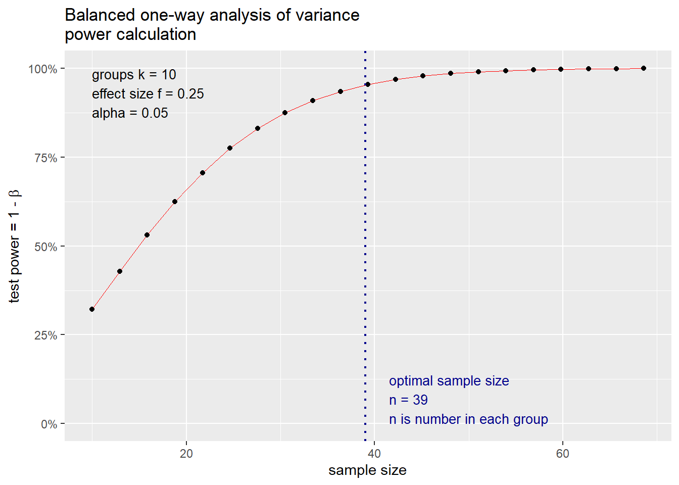
Figure 8.1: Visualization of power curve for one-way ANOVA example
Figure 8.1 depicts the power of the one-way ANOVA test as a function of the sample size per group \(n\). Similar graphics can also be produced in G\(^*\)Power. Although G\(^*\)Power allows the effect size \(f\) to be estimated using a table of \((\mu_i, n_i)\) values where the \(n_i\) values are not forced to be equal for all \(i = 1, ...,k\), G\(^*\)Power provides a common sample size recommendation for each group. The one-way ANOVA is called a balanced one-way ANOVA when \(n_1 = ... = n_k = n\). Finally, we note that neither the pwr package nor G\(^*\)Power provide functionality for sample size determination for one-way ANOVA when the within-group variance is not the same for all groups. We discuss how to conduct sample size calculations for such scenarios in Section 8.3.
8.2.4 Sample Size Determination for Multiple Regression Model
In this subsection, we focus on an omnibus \(F\)-test for multiple regression where we consider the deviation of \(R^2\) (the coefficient of determination) from 0. The multiple linear regression model explains the relationships between a dependent variable \(Y\) and \(p\) independent variables \(X_1\), …, \(X_p\). The type of multiple linear regression model explored in this subsection assumes that the independent variables are fixed. Thus, we consider a model for the response \(Y\) that is conditional on the values of the independent variables. Therefore, we assume that given \(N\) (\(\boldsymbol{Y}\), \(\boldsymbol{X}\))observations, \[\boldsymbol{Y} = \boldsymbol{X}\boldsymbol{\beta} + \boldsymbol{\varepsilon},\] where \(\boldsymbol{X} = [1, \boldsymbol{X}_1, ..., \boldsymbol{X}_p]\) is a \(N \times (p + 1)\) matrix of a constant term and fixed, known predictor \(\boldsymbol{X}_i\). Moreover, \(\boldsymbol{\beta}\) is a column vector of \(p + 1\) regression coefficients. The column vector \(\boldsymbol{\varepsilon}\) of length \(N\) contains the error terms such that \(\varepsilon_i \sim N(0, \sigma^2)\) for \(i = 1, ..., N\).
G\(^*\)Power supports power analyses for the test that the proportion of variance of the dependent variable \(Y\) explained by a set of predictors \(B = \{1, ..., p\}\), denoted \(R^2_{Y\cdot B}\), is equal to 0. The corresponding null and alternative hypotheses are \[H_0: R^2_{Y\cdot B} = 0 ~~~\text{vs.}~~~ H_A: R^2_{Y\cdot B} > 0.\] Under the null hypothesis, the appropriate test statistic follows an \(F\) distribution with \(p\) degrees of freedom in the numerator and \(N - (p+1)\) degrees of freedom in the denominator.
For this procedure, the effect size \(f^2\) is such that \(f^2 = V_S/V_E\), where \(V_S\) is the proportion of variance explained by the set of predictors \(B\), and \(V_E\) is the proportion of residual variance not explained by the predictors. That is, \(V_S + V_E = 1\). For the multiple linear regression scenario given above, the proportion of variance explained by the set of predictors \(B\) is given by \(R^2_{Y\cdot B}\) and the residual variance is given by \(V_E = 1 - R^2_{Y\cdot B}\). It follows that \[f^2 = \frac{R^2_{Y\cdot B}}{1 - R^2_{Y\cdot B}}.\]
G\(^*\)Power provides functionality to choose an effect size \(f^2\) using estimated correlations between the independent variables and the estimated correlations between the dependent variable \(Y\) and each independent variable. After users enter the number of independent variables \(p\) in their model, two Excel-type table appear. The first table is of dimension \(p \times 1\) and allows users to estimate a correlation coefficient between the response variable \(Y\) and each predictor variable. The second table is a matrix of dimension \(p \times p\), where users can estimate correlation coefficients between each pair of independent variables \((X_i, X_j)\) such that \(i < j\). We note that the correlation between \(X_i\) and itself is 1 and that the correlation coefficient for the pair of variables \((X_i, X_j)\) is symmetric in the roles of \(i\) and \(j\). After the user inputs these estimated values into the application, G\(^*\)Power returns an effect size \(f^2\). This process is explained in more detail on pages 33 and 34 of the G\(^*\)Power user manual. Users are also free to use the conventional effect sizes for the omnibus test for \(R^2\) with multiple linear regression as determined by Cohen (2013): \(f^2 =\) 0.02 for a small effect, 0.15 for a medium effect, and 0.35 for a large effect.
We now consider the following example. We suppose that we would like to consider a regression model with 5 independent variables, and we have reason to expect an effect size of \(f\) = 1/9. This is somewhere between a small and medium effect size. We now use the pwr.f2.test() function in the pwr package to determine the power that we have to detect this effect when \(\alpha\) = 0.05 and we have \(N =\) 95 observations. This example is also provided in the G\(^*\)Power user manual, so we will be able to compare the results from the two programs. The following R code conducts the sample size determination calculation for this example.
##
##      Multiple regression power calculation
##
##               u = 5
##               v = 89
##              f2 = 0.1111111
##       sig.level = 0.05
##           power = 0.6735858
For the pwr.f2.test() function, u is the degrees of freedom in the numerator, v is the degrees of freedom in the denominator, and f2 is the effect size. With these inputs, we estimate the power of the appropriate \(F\)-test to be 0.674. This is the same estimated power returned by G\(^*\)Power. The pwr package does not faciliate plotting power curves for the pwr.f2.test() function. This relatively simple multiple linear regression example exhausts the pwr package’s sample size determination capabilities. G\(^*\)Power provides much more functionality for sample size determination with regression models, including sample size calculations for comparing a single regression coefficient to a fixed value, sample size calculations for comparing the equality of two regression coefficients, and sample size calculations for considering the increase in the \(R^2\) value that arises from using a more complicated multiple linear regression model. These scenarios are described in the G\(^*\)Power user manual.
8.2.5 Sample Size Determination to Compare Two Means (Unknown, Common Variance)
In this subsection, we focus on a third and final scenario for sample size determination with the pwr package and G\(^*\)Power. For this scenario, we consider a \(t\)-test to gauge the equality of two independent populations means \(\mu_1\) (corresponding to group 1) and \(\mu_2\) (corresponding to group 2). The data consist of two samples of size \(n_1\) and \(n_2\) from two independent and normally distributed populations. For this test, we assume that the true standard deviations in the two populations are unknown and will be estimated from the data. The null and alternative hypotheses of this \(t\)-test are \[H_0: \mu_1 = \mu_2 ~~~\text{vs.}~~~ H_A: \mu_1 \ne \mu_2.\] We use a two-sided test if there is no restriction on the sign of the deviation of the alternative hypothesis \(H_A\). Otherwise, we use the one-sided test.
As mentioned earlier, the effect size in this scenario is \[d = \frac{\mu_1 - \mu_2}{\sigma},\] where \(\sigma\) is the common standard deviation for the two groups of normal data. Cohen (2013) suggested using \(d =\) 0.2 for a small effect, 0.5 for a medium effect, and 0.8 for a large effect. However, the effect size \(d\) for this situation is more interpretable than the effect sizes for the previous two scenarios considered. As such, researchers may have substantial enough information to choose an effect size for the sample size calculation.
We now consider the following example. We suppose that we would like to compare two means, and we expect to observe a “medium” effect size ( \(d\) = 0.5). We want to perform a two-sided hypothesis test to consider the equality of \(\mu_1\) and \(\mu_2\). We now use the pwr.t.test() function in the pwr package to determine how many observations we need in each group with \(\alpha\) = 0.05 to achieve a power of 0.8. The following R code conducts the sample size determination calculation for this example.
(p.t <- pwr.t.test(d=0.5, power=0.8, sig.level = 0.05, type = "two.sample",
                   alternative = "two.sided"))
##
## Two-sample t test power calculation
##
## n = 63.76561
## d = 0.5
## sig.level = 0.05
## power = 0.8
## alternative = two.sided
##
## NOTE: n is number in *each* groupFor the pwr.t.test() function, type can take a value of either "two-sample", "one-sample", or "paired". Moreover, alternative can take a value of "two.sided", "less", or "greater" – where "less" and "greater" should correspond to negative and positive values of d, respectively. After rounding the sample size up to the nearest integer, we determine that we require 64 observations per group for this example. For this example, we can return a power curve using the standard plot() function in R as demonstrated below in Figure 8.2.
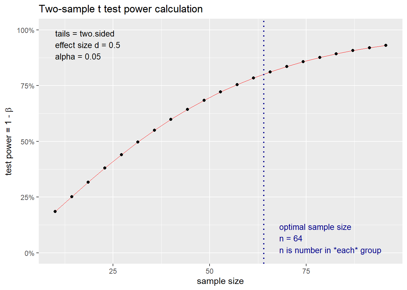
Figure 8.2: Visualization of power curve for two-sample t-test example
Figure 8.2 depicts the power of the two-sample \(t\)-test as a function of the sample size per group \(n\). Similar graphics can also be produced in G\(^*\)Power. The two-sample \(t\)-test functions in the pwr package force the standard deviation \(\sigma\) in the two groups to be the same. G\(^*\)Power does allow for sample size calculations where the standard deviations are not the same for the two groups (i.e., \(\sigma_1 \ne \sigma_2\)) for the case when \(n_1 = n_2\). However, this sample size determination calculation still assumes that Student’s t-test will be used, and this test assumes that the standard deviation is the same in both groups. Therefore, this sample size calculation facilitated by G\(^*\)Power is an approximate calculation. When \(\sigma_1 \ne \sigma_2\), it is more appropriate to use Welch’s t-test. Most free sample size determination software solutions do not offer this functionality, but we discuss how to conduct sample size calculations for this particular scenario in Section 8.3. We note that both the pwr package in R and G\(^*\)Power offer more sample size determination functionality than explored in the previous three examples. More details about this additional functionality can be found in the documentation for these software solutions.
8.2.6 The TOSTER Package
To conclude this subsection, we discuss the TOSTER package, which facilitates sample size calculations for equivalence tests when the TOST procedure is carried out using two one-sided \(t\)-tests. This package facilitates sample size determination for two-sample, one-sample, and paired \(t\)-tests, but we will focus on the two-sample case in this subsection. For the two-sample case, the TOSTER package requires that we make the assumption that the standard deviation \(\sigma\) is the same in both groups. For this scenario and a given equivalence margin \(\delta\), our null and alternative hypotheses are \[H_0: \{\mu_1 - \mu_2 \le -\delta\}\cup\{\mu_1 - \mu_2 \ge \delta\} ~~~\text{vs.}~~~ H_A: -\delta < \mu_1 - \mu_2 < \delta.\]
For this sample size determination calculation, we need to choose a values for the equivalence margin \(\delta\), the significance level \(\alpha\), and the power \(1 - \beta\); we must also estimate a value for the common standard deviation \(\sigma\) and estimate a value for \(\mu_1 - \mu_2\). The power_T_tost() function allows us to specify the true effect via the raw (unstandardized) effect. The power_t_TOST() function has the following arguments:
delta: the value fordeltais not the value specified for the equivalence margin \(\delta\). Instead, it is the value that we anticipate to observe for \(\mu_1 - \mu_2\). We can specifydeltausing the anticipated difference between \(\mu_1\) and \(\mu_2\). It is important to specify this difference because the power of the equivalence test is going to depend on how close the true value of \(\mu_1 - \mu_2\) is to either endpoint of the interval \((-\delta, \delta)\). If we anticipate that \(\mu_1 = \mu_2\), we may need less data to conclude practical equivalence than if \(\mu_1 - \mu_2\) is close to \(-\delta\) or \(\delta\).sd: the estimated value for the common standard deviation for the two groups.low_eqbound: the lower bound of the region of equivalence. This is typically \(-\delta\), but thepower_T_tost()allows for this interval to be asymmetric around 0.high_eqbound: the upper bound of the region of equivalence. This is typically \(\delta\), but thepower_T_tost()allows for this interval to be asymmetric around 0.alpha: the significance level for the test.power: the desired power of the equivalence test.
We now consider the following example. We suppose that we would like to compare two means, and we anticipate the difference between the two means to be 0.5. We anticipate that each group of data has a standard deviation of 5. Moreover, we define the equivalence margin to be 2 (i.e., it is not of practical importance if the means of the two groups differ by at most 2 in absolute value). We now use the power_t_TOST() function to determine how many observations we need in each group with \(\alpha\) = 0.05 to achieve a power of 0.8. The following R code conducts the sample size determination calculation for this example.
(p.TOST <- power_t_TOST(delta = 0.5, sd = 5, low_eqbound = -2, high_eqbound = 2,
                        alpha = 0.05, power = 0.8))
##
## Two-sample TOST power calculation
##
## power = 0.8
## beta = 0.2
## alpha = 0.05
## n = 140.3308
## delta = 0.5
## sd = 5
## bounds = -2, 2
##
## NOTE: n is number in *each* groupAfter rounding the sample size up to the nearest integer, we determine that we require 141 observations per group for this example. The TOSTER function does not support the plotting of power curves for equivalence tests. These curves must be plotted manually, as discussed in Section 8.3. The TOSTER package only supports basic sample size calculations for equivalence testing, but it is an accessible starting point in terms of software that is freely available.
8.3 Simulation-Based Sample Size Determination
8.3.1 Computing a Single Power Estimation via Simulation
If the model that we intend to use to analyze the data from the study is not supported by the pwr package in R or G\(^*\)Power, we may need to resort to simulation-based sample size determination. Simulation-based sample size determination involves specifying distributions for the data and generating samples of a given size \(n\). These samples of size \(n\) can typically be generated using built-in R functions – such as rnorm(), rexp(), rpois(), or rgamma(). For this simulated data, we conduct the hypothesis test of interest and record whether or not we reject the null hypothesis for a specified significance level \(\alpha\). We can repeat this process many times, and the proportion of simulations for which we reject the null hypothesis provides an estimate for the power of the test given the distribution(s) chosen for the data, the significance level \(\alpha\), and the sample size \(n\).
Simulation-based sample size determination can be useful in situations where heteroscedasticity is present (i.e., we have multiple groups of data, and the variance within each group is not the same). In these situations, we may not be able to compute the power of the statistical test using analytical formulas. Moreover, simulation-based sample size determination can also be useful when we would like to use nonparametric hypothesis tests. The pwr package does not provide any functionality for samples size calculations with nonparametric tests, and G\(^*\)Power offers very limited functionality.
We illustrate how to conduct simulation-based sample size determination using the following example. Let’s assume that we want to conduct a two-sample \(t\)-test, but we have reason to believe that the standard deviations from the two groups are not the same. Let’s assume that we want to conduct a two-sided hypothesis test. Let’s further assume that we believe that \(Y_{1j} \sim N(0, 1)\) for \(j = 1, ..., n_1\) and that \(Y_{2j} \sim N(1, 2)\) for \(j = 1, ..., n_2\). As such, we would anticipate using Welch’s \(t\)-test to conduct the hypothesis test. The Student’s two-sample \(t\)-test leverages a \(t\)-distribution with \(n_1 + n_2 - 2\) degrees of freedom. However, under the null hypothesis \(H_0: \mu_1 = \mu_2\) the Welch’s two-sample \(t\)-test has a \(t\)-distribution with the degrees of freedom given by \[df^* = \dfrac{\left(\frac{s_1^2}{n_1} + \frac{s_2^2}{n_2}\right)^2}{\frac{s_1^4}{n_1^2(n_1 -1)} + \frac{s_2^4}{n_2^2(n_2 -1)}},\] where \(s_1^2\) and \(s_2^2\) are the observed sample variance for the observations from groups 1 and 2. That is, we do not know the degrees of freedom for the test statistic a priori. This can make it difficult to compute the power of the \(t\)-test analytically. The following R code (with comments) shows how to estimate the power of Welch’s \(t\)-test in this scenario for \(n_1 = n_2 = 50\) and significance level \(\alpha = 0.05\) via simulation. This example assumes that the study design is balanced (i.e., \(n_1 = n_2\)), but this is certainly not a requirement for simulation-based sample size determination.
## choose the number of simulation repetitions
n_sim <- 1000

## set the significance level for the test
alpha <- 0.05

## set the sample size for each group
n1 <- 50
n2 <- 50

## set the anticipated parameters for each group
mu1 <- 0; sigma1 <- 1
mu2 <- 1; sigma2 <- 2

set.seed(1)
## initialize vector to output results of hypothesis test for simulated data
reject <- NULL
for (i in 1:n_sim){
  ## randomly generate simulated data from both groups
  y1 <- rnorm(n1, mu1, sigma1)
  y2 <- rnorm(n2, mu2, sigma2)

  ## conduct Welch's test (i.e., set var.equal = FALSE, which is the default)
  p.sim <- t.test(y1, y2, alternative = "two.sided", var.equal = FALSE)$p.value

  ## turn results into binary vector (1 if we reject null hypothesis; 0 otherwise)
  reject[i] <- ifelse(p.sim < alpha, 1, 0)
}

mean(reject)
## [1] 0.875Therefore, we estimate that Welch’s \(t\)-test has power of 0.875 to reject the null hypothesis \(H_0: \mu_1 = \mu_2\) when \(Y_{1j} \sim N(0, 1)\) for \(j = 1, ..., n_1\) and that \(Y_{2j} \sim N(1, 2)\) for \(j = 1, ..., n_2\) for \(n_1 = n_2 = 50\) and a signficance level of \(\alpha = 0.05\). For this simulation, we chose n_sim = 1000. This value ensures that the code runs quickly when compiling this document. We would likely want to use a larger value (at least n_sim = 10000) in practice. If we use small values for n_sim, then the estimated power will not be very precise. If \(\widehat{pwr}\) is a given estimate for the power of a hypothesis test in a given scenario, then the standard error of this estimate is given by
\[\sqrt{\frac{\widehat{pwr}(1 - \widehat{pwr})}{n_{sim}}}.\]
Therefore, if we choose n_sim = 10000, then the standard error of the estimate for power is at most 0.005 (this maximum is obtained when \(\widehat{pwr} =\) 0.5).
8.3.2 Estimating a Power Curve via Simulation
Both the pwr function in R and G\(^*\)Power facilitate the creation of power curves in certain scenarios. These power curves can also be estimated via simulation, although this may be a computationally intensive process. The following block of code takes the power estimation code from the previous code block. This function estPower() has eight inputs: the number of simulation repetitions n_sim, the sample sizes for each group n1 and n2, the anticipated parameters of the normal distribution for group 1 mu1 and sigma1, the anticipated parameters of the normal distribution for group 2 mu2 and sigma2, and the significance level alpha. This function can generally be used to conduct power analysis for two-sided Welch \(t\)-tests.
## put the previous code in functional form
estPower <- function(n_sim, n1, n2, mu1, sigma1, mu2, sigma2, alpha){
  ## initialize vector to output results of hypothesis test for simulated data
  reject <- NULL
  for (i in 1:n_sim){
    ## randomly generate simulated data from both groups
    y1 <- rnorm(n1, mu1, sigma1)
    y2 <- rnorm(n2, mu2, sigma2)

    ## conduct Welch's test (i.e., set var.equal = FALSE, which is the default)
    p.sim <- t.test(y1, y2, alternative = "two.sided", var.equal = FALSE)$p.value

    ## turn results into binary vector (1 if we reject null hypothesis; 0 otherwise)
    reject[i] <- ifelse(p.sim < alpha, 1, 0)
  }
  return(mean(reject))
}
The following R code demonstrates how to estimate and plot a power curve for this scenario. To estimate the power curve, we need to choose sample sizes at which to estimate the power of Welch’s \(t\)-test to reject the null hypothesis. For this example, we will restrict the sample size to be balanced for the two groups (\(n_1 = n_2\)). We choose the following 11 sample sizes at which to estimate the power of Welch’s test: 2, 5, 8, 10, 15, 20, 30, 40, 50, 60, and 75. The estimated power curve is plotted in Figure 8.3.
## choose the number of simulation repetitions
n_sim <- 1000

## set the significance level for the test
alpha <- 0.05

## set the sample size for each group (multiple values)
n1 <- c(2,5,8,10,15,20,30,40,50,60,75)
n2 <- c(2,5,8,10,15,20,30,40,50,60,75)

## set the anticipated parameters for each group
mu1 <- 0; sigma1 <- 1
mu2 <- 1; sigma2 <- 2

set.seed(2)
## initialize vector to output results of hypothesis test for simulated data
pwer <- NULL
for (j in 1:length(n1)){
  ## use helper function to estimate power
  pwer[j] <- estPower(n_sim, n1[j], n2[j], mu1, sigma1, mu2, sigma2, alpha)
}

plot(n1, pwer, type = "l", col = "firebrick", ylim= c(0,1),
     main = "Power curve for two-sided Welch test example", ylab = "Power",
     xlab = "Sample size (per group)")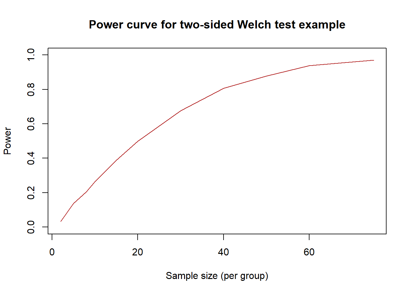
Figure 8.3: Visualization of power curve estimated via simulation
We note that the R code in this subsection could be modified to facilitate simulation-based sample size determination in other scenarios. The code above runs relatively quickly but the estimated power curve is not particularly smooth. To improve this, we may want to estimate the power of Welch’s test for more sample sizes than just the 11 that were considered above. Moreover, we would likely want to use a value of n_sim that is at least 10000 per estimate on the power curve. This suggests that estimating power curves via simulation can be a computationally intensive process. We discuss how to speed up this process in Section 8.3.3.
8.3.3 Parallelization for Simulation-Based Sample Size Determination
Parallelization can help make computing power curves or power estimates a faster process when one has access to a computer with multiple cores. Parallel computation structures the computing process such that many calculations or processes are carried out simultaneously. A large problem (computing a power curve) can often be divided into smaller ones (computing the various power estimates that comprise the power curve). These smaller problems can then be solved at the same time. The parallelization solution provided in this subsection leverages the foreach, doParallel, and doSNOW packages in R. The following R code shows how to estimate the power curve from Section 8.3.2 using parallel computing.
## load the required packages in this order
require(foreach)
require(doParallel)
require(doSNOW)

## set up the multiple cores for parallelization
## cores[1] returns the number of cores on your machine;
## this command makes a parallel computing environment with cores[1]-1 cores;
## this frees up a core to do other processes (do not assign more than cores[1]-1 cores).
cores=detectCores()
cl <- makeSOCKcluster(cores[1]-1)

## determine the number of parallel processes (the number of points on the power curve)
n_loop <- length(n1)

## choose the number of simulation repetitions
n_sim <- 1000

## set the significance level for the test
alpha <- 0.05

## set the sample size for each group (multiple values)
n1 <- c(2,5,8,10,15,20,30,40,50,60,75)
n2 <- c(2,5,8,10,15,20,30,40,50,60,75)

## set the anticipated parameters for each group
mu1 <- 0; sigma1 <- 1
mu2 <- 1; sigma2 <- 2

## this code sets up a progress bar; this is helpful if you have less than n_loop
## cores available (you can see the proportion of the smaller tasks that have been completed)
registerDoSNOW(cl)
pb <- txtProgressBar(max = n_loop, style = 3)
progress <- function(n) setTxtProgressBar(pb, n)
opts <- list(progress = progress)

## the foreach() function facilitates parallelization (described below)
pwer2 <- foreach(j=1:n_loop, .combine="c", .packages = c("foreach"),
                               .options.snow=opts) %dopar% {
                                 set.seed(j)

                                 ## function outputs the estimated power for each
                                 ## point on the curve (from previous code block)
                                 estPower(n_sim, n1[j], n2[j], mu1, sigma1, mu2, sigma2, alpha)
                               }
The previous code block can be used to reproduce the estimated power curve from earlier (just replace pwer with pwer2 in the plot command). The foreach() function faciliates the parallelization for this example. We discuss several of its important arguments below:
j: this input should take the form1:n_loop, wheren_loopis the number of tasks that must be computed in parallel..combine: this argument denotes how the objects returned by each parallel task should be combined. Specifying"c"will concatentate these results into a vector, and usingcbindorrbindcan be used to combine vectors into a matrix. For this example, each parallel task returns a single power estimate, so we selected"c"..packages: this argument should be a character vector denoting the packages that the parallel tasks depend on. For this situation, we do not need the foreach package to compute the power estimates, but this shows the format that this argument must take if we do have any dependencies for the parallel tasks.options.snow: this argument sets up the progress bar. As long asn_loopis modified as necessary, we do not need to change any other code associated with the progress bar to modify this code for a different example..errorhandling: this argument is set tostopby default. This means that if one of the cores encounters an error message when computing a smaller task, the execution of all tasks is stopped. We recommend using this default setting so that you are alerted to the issue and can investigate potential problems with the code.
If you have a very computationally intensive sample size calculation, you can run your code on the MFCF servers for graduate students, faculty, and staff in the Math Faculty. You should have up to 72 cores available when using the MFCF servers, which is likely more computing power than is available on a desktop computer.
Finally, the above code block computed the power estimate for each point on the power curve using a regular for loop. Each of the estimates on the power curve were computed in parallel. If it takes a very long time to compute a single power estimate, then you may want to compute each power estimate in parallel and iterate through all power estimates on the curve using a regular for loop. This could be done by modifying the code block above. We could replace estPower() with a function that returns a binary result to denote whether the null hypothesis was rejected for a single simulation run. We would want to then specify j=1:n_sim for the foreach() function call, and then we would wrap this foreach() function call in a regular for loop from i = 1:n_loop. We note that it is certainly not necessary to parallelize a sample size calculation, but it can be helpful if the calculation is very computationally intensive.
8.4 Beyond Sample Size Determination
Sound experimental design does not end with sample size determination. It can be helpful to discuss concepts that are related to sample size determination with the researcher. For instance, maybe the researcher has decided that they would like to collect 50 observations per group for the two groups in their study. In this situation, it would be a good idea to discuss randomization with the researcher. It is not ideal to simply assign the first 50 observations to the first treatment and the last 50 observations to the second treatment.
There may also be situations where a researcher might want to collect a smaller sample than recommended and then decide whether or not to collect a larger sample based on the results from analyzing the smaller sample. This is related to the statistical concept of peeking, where we monitor the data as they are observed and decide whether to continue or stop the experiment. It is not ideal to observe the data in stages, but it should be disclosed as part of the analysis that the data were not observed all at once if the data from both samples is used as part of the study.