5 Introduction to Nonparametric Statistics
Author: Kelly Ramsay
Last Updated: Nov 10, 2020
5.1 Introduction
The aim of this chapter is to introduce nonparametric analogues of common statistical methods including ANOVA, two-sample tests, confidence intervals, and regression. Nonparametric statistical methods impose fewer assumptions on the data than their parametric counterparts. Some reasons for using nonparametric methods include:
- the data appear to be non-normal, or do not appear to fit the appropriate parametric assumptions for the problem;
- the sample size is too small for certain large sample approximations;
- the analyst is not comfortable imposing the typical model assumptions on the data; and
- the data contains outliers. (This reason only applies to rank-based methods, which are more resistant to outliers.)
The benefits of nonparametric statistics do not come for free. When the assumptions of a parametric model are satisfied, the parametric model-based procedures are typically more accurate/powerful. However, we cannot know for sure if those assumptions are satisfied.
5.1.1 R Packages and Data
In this chapter, the following libraries will be used:
These packages can be installed using the install.packages() function as mentioned in Introduction to R.
Throughout this document, we will use the iris data as an example.
##   Sepal.Length    Sepal.Width     Petal.Length    Petal.Width
##  Min.   :4.300   Min.   :2.000   Min.   :1.000   Min.   :0.100
##  1st Qu.:5.100   1st Qu.:2.800   1st Qu.:1.600   1st Qu.:0.300
##  Median :5.800   Median :3.000   Median :4.350   Median :1.300
##  Mean   :5.843   Mean   :3.057   Mean   :3.758   Mean   :1.199
##  3rd Qu.:6.400   3rd Qu.:3.300   3rd Qu.:5.100   3rd Qu.:1.800
##  Max.   :7.900   Max.   :4.400   Max.   :6.900   Max.   :2.500
##        Species
##  setosa    :50
##  versicolor:50
##  virginica :50
##
##
##
This data set contains 4 continuous variables, namely Sepal.Length, Sepal.Width, Petal.Length and Petal.Width. The variable Species is a Categorical variable.
Other examples used in this chapter will involve simulated data sets.
5.1.2 Sample Ranks
Many nonparametric procedures rely on ranking the data. Ranking a data variable means putting the values in order, from smallest to largest. Each point is then assigned a number for where in the order they fall. For example, the smallest observation has rank 1, the second smallest has rank 2, etc. the largest has rank \(n\).
## [1] -0.27962018 0.02912338 0.62909474 0.47840529 -0.79437766## [1] 2 3 5 4 15.1.3 Sampling Distribution
Probability distributions are often understood by researchers in the context of “What is the distribution of my data?”.
In statistical analysis, we should also be concerned with the distribution of any estimators computed from the data. An estimator is a quantity that is computed from the data to estimate a population quantity, such as the sample mean (used to estimate the population mean) and the sample variance (used to estimate the population variance).
The distribution of an estimator, known as its sampling distribution, gives the researcher a measure of how the estimator would vary across different samples drawn from the population. The sampling distribution allows the researcher to quantify the error introduced by the fact that different samples give different estimates of the population values.
For example, one thing we might estimate is a population mean \(\mu\), which can be estimated using the sample mean \(\bar{x}\). The estimator here is then the sample mean. For large \(n\) (sample size) and independent data, \(\bar{x}\) is normally distributed with mean \(\mu\) and variance \(\sigma^2/n\), where \(\sigma^2\) is the variance of the population. This is the sampling distribution of \(\bar{x}\). We then use the quantiles of this sampling distribution to construct confidence intervals for the population parameter.
5.2 Two-sample Hypothesis Testing
5.2.1 Quick Reference Table
| Observation type | Test goal | Test |
|---|---|---|
| Independent | Difference in Mean | Wilcoxon rank-sum |
| Paired | Difference in Mean | Wilcoxon sign |
| Independent | Difference in Variance | Tukey-Siegel |
| More than two groups | - | See ANOVA |
5.2.2 Wilcoxon Rank-Sum Test
The Wilcoxon rank-sum test, also known as the Mann-Whitney U test, is used to test for a difference between two groups of observations. The null and alternate hypotheses for this test are: \[ H_0\colon \tx{Both groups have the same distribution. vs. } H_1\colon\ \tx{One group stochastically dominates another.} \] Assumptions:
- The variable of interest is continuous or ordinal.
- Data has only two groups.
- All observations are independent.
Notes:
- The alternative is that in essence, the groups differ. One can read about stochastic domination here.
- If the analyst is willing to assume that the distributions of each group have the same shape and scale/variance, then the alternative becomes “The group’s median differs.”
- If both groups are normal, then this is also a test for a difference in means.
- Mathematically, the test works if \(P(X_1-X_2<0)\neq 1/2\) if \(X_1\) and \(X_2\) are random observations from groups 1 and 2 respectively.
5.2.2.1 Test Concept
To perform the Wilcoxon rank-sum test, we must rank the response from lowest to highest, over both samples; both samples are pooled together and then the data is ranked.
The Wilcoxon rank-sum test relies on the intuition that if the two groups have the same distribution then they should have, on average, the same amount of high and low ranked variables.
The test checks to see if one group has an abnormally large amount of high-ranked variables.
5.2.2.2 An example using R
We use the iris data as an example, in which our focus is the two species setosa and versicolor
# first two iris species
iris2 <- iris[1:100, ]
# for clean graph, can be ignored
iris2[, 5] <- as.factor(as.character(iris[1:100, 5]))


boxplot(Sepal.Length ~ Species, xlab = "Species", data = iris2)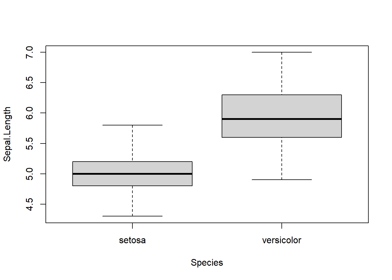
Figure 5.1: Boxplots of sepal length by species.
Notice that the medians appear to be quite different for the two species, so we expect to reject the rank-sum test. We also notice that each group seems to have approximately the same shape and spread. This would allow us to interpret a rejected rank-sum test as the groups have different medians.
We can use the wilcox_test() function in the coin package to perform the Wilcoxon rank-sum test. The function wilcox_test() first takes a formula of the form response_variable ~ group_variable. It also has a data argument to specify the data frame that contains the group and response variable.
# iris[1:100,] is the first two species in the data
coin::wilcox_test(Sepal.Length ~ Species, data = iris[1:100, ])
##
## Asymptotic Wilcoxon-Mann-Whitney Test
##
## data: Sepal.Length by Species (setosa, versicolor)
## Z = -7.4682, p-value = 8.13e-14
## alternative hypothesis: true mu is not equal to 0The output contains the test statistic and \(p\)-value. At the end of the output, notice that we do reject the hypothesis of the same distribution.
5.2.4 Wilcoxon Signed Rank Test
The Wilcoxon signed-rank test is used to test for a difference in rank means between observations when the data can be paired. The null and alternate hypotheses are: \[ H_0\colon \tx{The median difference between the groups is 0. vs. } H_1\colon\ \tx{The groups have different medians.} \] Assumptions:
- The variable of interest is continuous or ordinal.
- Data has only two groups.
- The between-subject observations are independent.
- The within-subject/within-pair observations can be dependent.
- The distribution of each group is symmetric. If this is not satisfied, the test will still work, but the null and alternative hypotheses would be \(H_0\colon\) The groups have the same distribution. vs. \(H_1\colon\) The groups have different distributions.
5.2.4.1 Test Concept
In the Wilcoxon signed-rank test, the absolute differences between pairs are ranked, rather than the observations themselves.
The idea is that if there is a difference between the two groups then the absolute differences should be large. The sign of the difference is also accounted for, since we expect the sign of the differences to be consistent one way another. For example, if the paired observations correspond to time 1 and time 2, and if the mean of time 2 is higher, then we expect the differences (time2-time1) to be positive more often than not.
5.2.4.2 An example using R
We will simulate a set of paired data set to demonstrate how to conduct the Wilcoxon Rank-Sum Test.
# Create a fake paired data set, this code simply creates an example of a data set where the observations are associated.
before <- rnorm(100, 2)
after <- before * .2 + rnorm(100, 1)
test_data <- data.frame(before, after)

# Boxplot of simulated data
boxplot(test_data)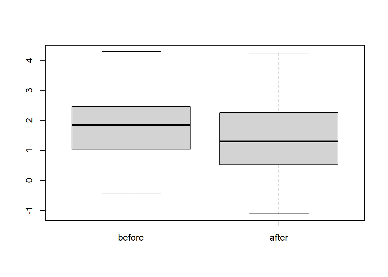
Figure 5.2: Boxplot of simulated paired data.
The boxplots show that the two medians are quite different. Hence, we expect to reject this test. Notice whiskers of both boxplots are symmetric, so it is reasonable to agree that the assumptions required for the signed-rank test are satisfied.
We can use the wilcoxsign_test() function in the coin package to perform the Wilcoxon rank-sum test. The function wilcoxsign_test() first takes a formula of the form response_variable ~ group_variable. It also has a data argument where you specify your data frame that contains your group variable and your response variable.
##
##  Asymptotic Wilcoxon-Pratt Signed-Rank Test
##
## data:  y by
##   x (pos, neg)
##   stratified by block
## Z = 2.6991, p-value = 0.006953
## alternative hypothesis: true mu is not equal to 0
The test statistic and \(p\)-value of the tests are reported. They indicate that the null hypothesis is indeed rejected.
Notes:
- This test also has an option zero.method which specifies the way zero differences are handled.
- The default method is the "Pratt" method, which has been shown to be a better method of handling zeros than the traditional Wilcoxon test.
- If you compute the Wilcoxon sign test with another software you may get a slightly different answer.
5.2.5 Siegel-Tukey Test
The Siegel-Tukey test is akin to the Wilcoxon rank-sum test, but the goal is to test for a difference in variance/dispersion between two groups.
5.2.5.1 Hypotheses
\[ H_0\colon \tx{Both groups have the same variance. vs. } H_1\colon\ \tx{Both groups do not have the same variance.} \] Assumptions:
- Variable of interest is continuous or ordinal.
- Data has only two groups.
- All responses are independent.
- Groups have the same mean or median. One can subtract each group’s respective median to meet this assumption.
5.2.5.2 Test Concept
To perform the Siegel-Tukey test we must rank the responses by how extreme the observation is, rather than how large.
Intuitively, if one group has a larger variance then it will have a larger amount of observations that are high and low relative to the median.
The test checks to see if one group has a large number of extreme observations.
5.2.5.3 An Example Using R
We can use the siegelTukeyTest() function in the PMCMRplus package to perform the Siegel-Tukey test. The function siegelTukeyTest() takes the first sample and second sample as its two arguments. In this example, we will use simulated data to demonstrate the use of the function.
# s1 and s2 have the same variance and mean
s1 <- rnorm(100, sd = 2)
s2 <- rnorm(100, sd = 2)
boxplot(s1, s2)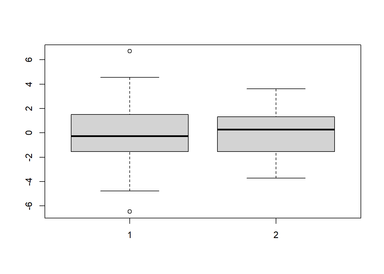
Figure 5.3: Boxplots of data from distributions with the same variance.
##
##  Siegel-Tukey rank dispersion test
##
## data:  s1 and s2
## W = 4611, p-value = 0.3433
## alternative hypothesis: true ratio of scales is not equal to 1
# s1 and s2 are random samples with different variances but the same mean
s1 <- rnorm(100, sd = 3)
s2 <- rnorm(100, sd = 2)
boxplot(s1, s2)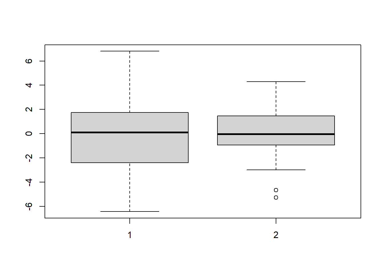
Figure 5.4: Boxplots of data from distributions with different variances.
##
##  Siegel-Tukey rank dispersion test
##
## data:  s1 and s2
## W = 3299, p-value = 2.648e-05
## alternative hypothesis: true ratio of scales is not equal to 1
# s1 and s2 are random samples with different variances but with different means
s1 <- rnorm(100, m = 4, sd = 3)
s2 <- rnorm(100, m = 0, sd = 2)
boxplot(s1 - median(s1), s2 - median(s2))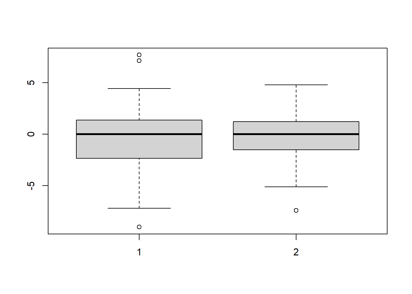
Figure 5.5: Boxplots of data from distributions with different variances.
# notice we subtract the medians
# We expect to reject here
PMCMRplus::siegelTukeyTest(
  x = s1 - median(s1),
  y = s2 - median(s2)
)
##
## Siegel-Tukey rank dispersion test
##
## data: s1 - median(s1) and s2 - median(s2)
## W = 4168, p-value = 0.04201
## alternative hypothesis: true ratio of scales is not equal to 1The reported test statistic and \(p\)-value agrees with our expectations in both examples.
5.3 ANOVA-type Methods
5.3.1 One-way ANOVA
We can start with introducing nonparametric one-way ANOVA. We apply ANOVA to test whether or not there is a difference in a response/dependent variable between different groups. The nonparametric equivalent of the ANOVA \(F\) test is the Kruskal-Wallis rank test or KW test for short.
The KW test does not require a distributional assumption on the data; the data need not be normal in order for the test to be valid. Additionally, since this test is based on ranks, it is also robust to extreme observations and/or outliers in the data. These are both valid justifications for using Kruskal-Wallis ANOVA.
The null and alternate hypotheses are:
\[ H_0\colon \tx{All groups have the same distribution. vs. } \\ H_1\colon\ \tx{At least one group stochastically dominates another.} \] Assumptions:
- The response variable is continuous or ordinal.
- Data has more than 2 groups (see here for two-group methods.).
- All responses are independent.
Notes:
- The alternative is that in essence, one group differs from the others. One can read about stochastic domination here.
- If the analyst is willing to assume that the distributions of each group have the same shape and scale/variance, then the alternative becomes “At least one group’s median differs.”
- Under standard parametric ANOVA assumptions, the standard parametric ANOVA hypotheses are covered by these hypotheses. In other words, if the data are normal with the same variance, then this is also a test for a difference in means.
- Let \(g\) be the number of groups. Mathematically, if \(p_j\) is the proportion of observations in group \(j\), and \(X_j\) is a random observation from group \(j\), then the test works if \(\sum_{j=1}^g p_jP(X_i-X_j<0)\neq 1/2\) for at least one group \(i\). This can generally be interpreted as the median differences \(X_i-X_j\) between groups being non-zero for some pairs of groups.
5.3.1.1 Test Concept
To perform KW ANOVA, the response values are ranked from lowest to highest, regardless of group.
KW ANOVA relies on the intuition that a group which has a higher response on average, when compared to the remaining groups, will then have higher ranks on average as well. Conversely, if the groups all have the same distribution, we expect them to have roughly equal high and low-ranked responses.
Therefore, the hypothesis is rejected if one or more groups have a disproportionately large amount of high or low ranked responses.
5.3.1.2 An Example Using R
We again use the iris data as an example.
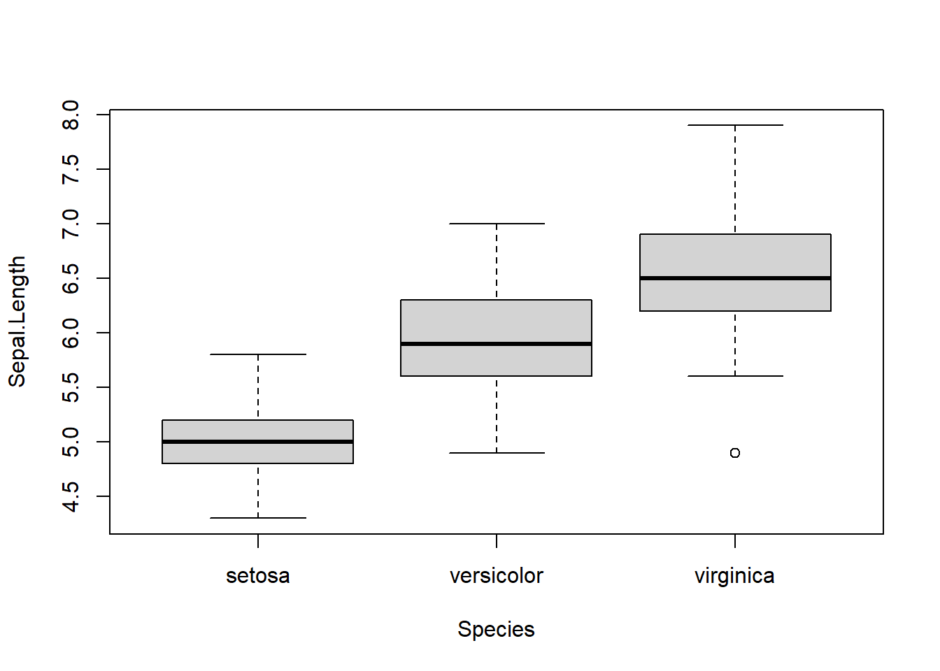
Figure 5.6: Boxplots of petal length by species.
par(mfrow = c(1, 3))
hist(iris[1:50, ]$Sepal.Length, xlim = c(3, 9), breaks = 15, xlab="setosa", main="")
hist(iris[51:100, ]$Sepal.Length, xlim = c(3, 9), breaks = 15, xlab="versicolor", main="")
hist(iris[101:150, ]$Sepal.Length, xlim = c(3, 9), breaks = 15, xlab="virginica", main="")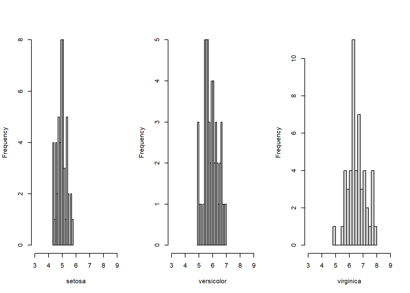
Figure 5.7: Histograms of sepal length for each species.
We see that the medians of the species are quite different, so we expect to reject the Kruskal-Wallis test. Notice that the distributions are approximately symmetric, and have a similar variance. This allows us to interpret the Kruskal-Wallis test as a test for a difference in medians. We can now run the KW Anova.
The kruskal.test() and the kruskal_test() functions are used to perform KW ANOVA. The coin package must be installed to use kruskal_test(). Both kruskal.test() and kruskal_test() have a data argument to specify the data frame that contains the group variable and the response variable. They also have a formula argument which should be in the form response_variable ~ group_variable.
Suppose we want to test whether the different species of iris flowers have different mean petal lengths. Here, Petal.Length is the response variable and Species is the group variable. These variables are stored in the iris data frame, and so we set the data argument to iris.
##
##  Kruskal-Wallis rank sum test
##
## data:  Petal.Length by Species
## Kruskal-Wallis chi-squared = 130.41, df = 2, p-value <
## 2.2e-16##
## Asymptotic Kruskal-Wallis Test
##
## data: Petal.Length by
## Species (setosa, versicolor, virginica)
## chi-squared = 130.41, df = 2, p-value < 2.2e-16The test outputs the test statistic (130.41) and the \(p\)-value (< 2.2e-16).
Under the null hypothesis, the KW test statistic follows a Chi-Squared distribution with \(\# \text{of groups}-1\) degrees of freedom. Here, there are 3 groups so the degrees of freedom (df) is 2 (=3-1).
The function kruskal.test() relies on an asymptotic approximation of the null distribution, which is appropriate if each group has at least 5 observations.
5.3.1.3 Notes
- For small samples, say each group has around 5 or fewer observations, it is recommended to use
kruskal_test()function with thedistributionargument set to"approximate". The"approximate"method uses a Monte Carlo approximation of the null distribution rather than relying on a large sample argument, but takes longer computationally.
##
##  Approximative Kruskal-Wallis Test
##
## data:  Petal.Length by
##   Species (setosa, versicolor, virginica)
## chi-squared = 130.41, p-value < 1e-04- As mentioned in the assumptions, the response/dependent variable should be continuous or can be approximated by a continuous variable. For example, Likert scale values are not continuous but they can be approximated by a continuous variable which can take any value between 1 and 5. Another variable that can be approximated by a continuous one is age.
- The categories should not be ordered; the group variable should not be ordinal.
- Sometimes responses will have the same value, resulting in tied ranks. A good method is to assign the tied observations the middle rank if they had not been tied. For example if the data are \(\{1,2,2,3\}\) the observations would be assigned ranks \(\{1,2.5,2.5,4\}\). This is done automatically in the
kruskal_test()function. Note that ties have been shown to have a small influence unless there are many ( say > 25%) ties. If many ties are present, we recommend using the procedure discussed in Note 1. to compute the \(p\)-value.
5.3.2 Post Hoc Comparisons for KW ANOVA
When the KW Anova is rejected, we may then want to find which pairs of groups are different from each other. These are called post-hoc comparisons.
After a significant KW result, we can use Dunn’s test to compute post-hoc pairwise comparisons. Dunn’s test checks for significant differences in pairwise rank means, given that a significant result was seen in the KW test.
5.3.2.1 Hypotheses
\[ H_0\colon \tx{Groups have the same distribution. vs. } H_1\colon\ \tx{One group stochastically dominates the other.} \]
5.3.2.2 An Example Using R
Now that we have seen a significant KW Anova result with the iris data, we would like to see between which species there exist differences. Given the boxplots, we expect all 3 pairwise comparisons to be significant.
The Dunn test is done via the package and function which are both named dunn.test. The dunn.test() function takes two arguments, the first is the response variable and the second is the group variable.
To adjust for running multiple hypothesis tests, we can use the method argument to account for the increased probability of type 1 error. Popular options include "none", "bonferroni" "sidak "bh".
The alpha argument adjusts the overall significance level of the tests, if the method argument is "none" then this is the significance level of each pairwise test. To read more about \(p\)-value adjustments and the multiple testing problem, see here, here and here.
##   Kruskal-Wallis rank sum test
##
## data: x and group
## Kruskal-Wallis chi-squared = 130.411, df = 2, p-value = 0
##
##
##                            Comparison of x by group
##                                 (No adjustment)
## Col Mean-|
## Row Mean |     setosa   versicol
## ---------+----------------------
## versicol |  -5.862996
##          |    0.0000*
##          |
## virginic |  -11.41838  -5.555388
##          |    0.0000*    0.0000*
##
## alpha = 0.05
## Reject Ho if p <= alpha/2## Kruskal-Wallis rank sum test
##
## data: x and group
## Kruskal-Wallis chi-squared = 130.411, df = 2, p-value = 0
##
##
## Comparison of x by group
## (Benjamini-Hochberg)
## Col Mean-|
## Row Mean | setosa versicol
## ---------+----------------------
## versicol | -5.862996
## | 0.0000*
## |
## virginic | -11.41838 -5.555388
## | 0.0000* 0.0000*
##
## alpha = 0.05
## Reject Ho if p <= alpha/2# changing significance level
dunn.test::dunn.test(iris$Petal.Length, iris$Species, method = "bh", alpha = 0.01)## Kruskal-Wallis rank sum test
##
## data: x and group
## Kruskal-Wallis chi-squared = 130.411, df = 2, p-value = 0
##
##
## Comparison of x by group
## (Benjamini-Hochberg)
## Col Mean-|
## Row Mean | setosa versicol
## ---------+----------------------
## versicol | -5.862996
## | 0.0000*
## |
## virginic | -11.41838 -5.555388
## | 0.0000* 0.0000*
##
## alpha = 0.01
## Reject Ho if p <= alpha/2The output includes a redo of the KW test (first sentence), the output of the Dunn test (the table), the significance level (alpha), and the rejection rule.
Each cell in the outputted table contains the Dunn test statistic followed by the \(p\)-value for the pairwise comparison between the cell row and cell column. A * is placed beside the \(p\)-value if a comparison is significant.
We can also do many to one comparisons, using the kwManyOneDunnTest() function in the PMCMRplus package.
Suppose we are only interested in whether the versicolor species and virginica species differ from the setosa species. Many-to-one comparisons are for when we are only interested in differences with one group, say the control.
The kwManyOneDunnTest() function has a formula argument where a formula in the form response_variable ~ group_variable is specified. The groups are compared with the first group listed in the group variable so your data may need to be reordered. In other words, the group representing “one” in the term “many to one” should be listed first.
The data argument is the data frame that contains the variables in the formula argument.
The alternative argument can be used to choose the type of alternative hypothesis between "two.sided" "greater" "less".
The p.adjust.method argument can be used to adjust for running multiple hypothesis tests; it is used to account for the increased probability of type 1 error.
Some options include "bonferroni", "BH", "fdr", and "none".
For a full list run the line ?PMCMRplus::frdAllPairsExactTest to get the help page for this function. To read more about \(p\)-value adjustments and the multiple testing problem, see here, here and here.
## Warning in kwManyOneDunnTest.default(c(1.4, 1.4, 1.3, 1.5, 1.4, 1.7,
## 1.4, : Ties are present. z-quantiles were corrected for ties.
##
## Pairwise comparisons using Dunn's many-to-one test## data: Petal.Length by Species## setosa
## versicolor 9.1e-09
## virginica < 2e-16##
## P value adjustment method: single-step## alternative hypothesis: two.sidedEach row contains the \(p\)-value for the comparison between the setosa group and the group name for that row.
5.3.3 Repeated Measures ANOVA (Friedman Test)
Repeated measures data are data such that the response is measured multiple times per subject. For example, a subject is given each treatment and the response is measured once for each treatment. Treatments can refer to time periods or other grouping variables. We can use the Friedman test on this type of data.
5.3.3.1 Hypotheses
\[ H_0\colon \tx{All treatment groups have the same distribution.vs. } \\ H_1\colon\ \tx{At least one treatment group does not have the same distribution.} \]
Assumptions:
- The response/dependent variable should be continuous or can be approximated by a continuous variable.
- Data has more than two treatments/groups/time periods (see here for two periods only).
- Subjects are independent.
- Within-subject measurements can be dependent.
- There are an equal number of measurements per subject/block. If this does not hold for your data, but the other assumptions do, see the Durbin test. See the Note 2. below.
Notes:
- If the groups have similar shapes and scales, then the Friedman test tests for a difference in medians between the groups.
5.3.3.2 Test Concept
We can use the Friedman test to perform a repeated-measures ANOVA. The Friedman test relies on the same intuition discussed in the KW ANOVA section; no differences between the groups should imply that there are roughly equal high and low ranks within each group.
The difference between the Friedman test and the KW test is that ranks are now computed within-subjects instead of across subjects, to account for intrasubject dependencies.
5.3.3.3 An Example Using R
We create some sample repeated measures data below.
It appears that the medians at each treatment are different from each other. According to the boxplots, the shape and scale of the distributions are similar, and so we can interpret a Friedman test as testing for a difference in medians.
set.seed(440)
# Create a fake repeated measures data set
# Note it is not necessary to understand how to simulate a data set in order to apply Friedman ANOVA, so this code block is optional.
time_0 <- rnorm(100, 2)
time_1 <- time_0 * .2 + rnorm(100, 1) # time 1 observation has a dependency on the time 0 observation.
time_2 <- time_1 * .2 + rnorm(100, 3) # time 2 has dependency on time 1, which implies dependency on time 0

# Putting the data in the above format
resp <- c(time_0, time_1, time_2) # create response variable
subj <- as.factor(rep(1:100, 3)) # create subject variable
tmnt <- as.factor(rep(1:3, each = 100)) # create treatment or time variable
test_data <- data.frame(resp, subj, tmnt) # put variables in data frame

# This fake data set has dependencies when the subject number is the same. We expect to reject this Friedman test since the mean at time 3 is 3.28, the mean at time 2 is 1.4 and the mean at time 1 is 2.

boxplot(test_data$resp ~ test_data$tmnt)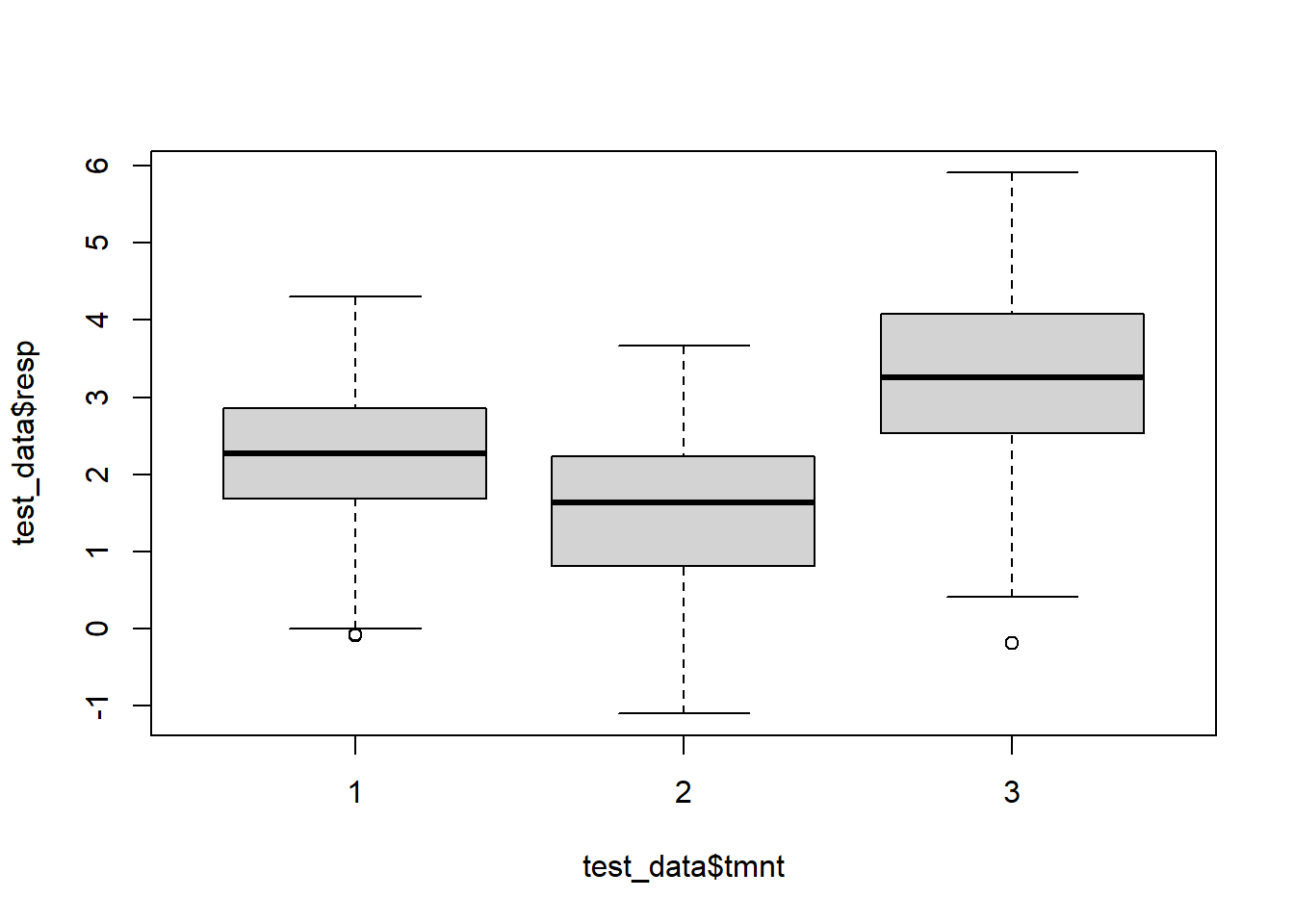
Figure 5.8: Boxplots of simulated responses from three different groups.
The `friedman_test() function is used to perform nonparametric repeated-measures ANOVA.
friedman_test() has a data argument where you specify your data frame that contains your treatment variable, subject variable, and your response variable. Data should be in the following format:
| Response | Subj | Treatment |
|---|---|---|
| .25 | 1 | 1 |
| .25 | 1 | 2 |
| .25 | 1 | 3 |
| .25 | 2 | 1 |
| … | … | … |
The friedman_test() function takes a formula in the form response_variable ~ treatment_variable|subject variable.
##
##  Asymptotic Friedman Test
##
## data:  resp by
##   tmnt (1, 2, 3)
##   stratified by subj
## chi-squared = 92.94, df = 2, p-value < 2.2e-16
# For "small" samples set distribution="approximate"
coin::friedman_test(resp ~ tmnt | subj, test_data, distribution = "approximate")##
## Approximative Friedman Test
##
## data: resp by
## tmnt (1, 2, 3)
## stratified by subj
## chi-squared = 92.94, p-value < 1e-04For small samples, see Note 1. in the Kruskal-Wallis ANOVA section.
5.3.4 Post Hoc tests
The package PMCMRplus contains many types of rank-based ANOVAs and post-hoc tests.
We will cover the exact test, but other tests may be used. The exact test checks for significant differences in pairwise rank means, given that a significant result was seen in the Friedman test.
5.3.5 An example using R
We will continue with our fake data.
Suppose we want to compute all pairwise differences, to see between which groups there were differences. To compute all pairwise comparisons, use the frdAllPairsExactTest() function in the PMCMRplus package.
The first argument y takes the response values, the second argument groups takes the group or treatment values and the third argument blocks takes the subject or block values.
To adjust for running multiple hypothesis tests, we can use the p.adjust.method argument to account for the increased probability of type 1 error.
Some options include "bonferroni", "BH", "fdr", and "none".
For a full list run the line ?PMCMRplus::frdAllPairsExactTest to get the help page for this function. To read more about \(p\)-value adjustments and the multiple testing problem, see here, here and here.
PMCMRplus::frdAllPairsExactTest(test_data$resp, test_data$tmnt, test_data$subj, p.adjust.method = "none")##
## Pairwise comparisons using Eisinga, Heskes, Pelzer & Te Grotenhuis all-pairs test with exact p-values for a two-way balanced complete block design## data: y, groups and blocks## 1 2
## 2 0.00033 -
## 3 1.6e-09 < 2e-16##
## P value adjustment method: noneThe \(p\)-values are given within cells, each cell corresponds to a comparison of the treatments corresponding to the cell’s row and the cell’s column. For example, the upper-left cell says that the \(p\)-value for testing a difference of rank means between the first and second treatment is 0.00033.
Instead of doing all comparisons, we can also do many-to-one comparisons. The frdManyOneExactTest() function compares all treatments to the first treatment listed in the treatment variables and takes the same arguments as frdAllPairsExactTest().
PMCMRplus::frdManyOneExactTest(test_data$resp, test_data$tmnt, test_data$subj, p.adjust.method = "none")##
## Pairwise comparisons using Eisinga-Heskes-Pelzer and Grotenhuis many-to-one test for a two-way balanced complete block design## data: y, groups and blocks## 1
## 2 0.00033
## 3 1.6e-09##
## P value adjustment method: none## alternative hypothesis: two.sidedEach row has a \(p\)-value that corresponds to the comparison of a group with group 1.
Notes:
- If you are looking for a specific non-parametric test not discussed here, it is likely in the PMCMRplus package and you may find that test here.
- The Friedman test assumes that there are equal numbers of observations within each block. For incomplete block designs, the Durbin test can be used. This can be done in R with the
durbinTest()function in the PMCMRplus package.
5.4 Boostrap Methods
Before proceeding, if the reader is not familiar with the term sampling distribution, then it is useful to read the section on sampling distributions.
5.4.1 Bootstrap Confidence Intervals
When computing confidence intervals for an estimated value, such as mean or regression parameter, typically we rely on the fact that the sampling distribution of the estimated value is normal. The estimated value is normally distributed for large \(n\).
The confidence interval is then of the form \[\hat{\theta}\pm Z_{1-\alpha/2}s_n,\] where \(s_n\) is the standard error and \(Z_{1-\alpha/2}\) is the \(1-\alpha/2\)-quantile or percentile of the normal distribution.
The key concept here is that \(\hat{\theta}\) is approximately normally distributed with mean \(\theta\) and variance close to \(s_n^2\). This means that the variability or error in our estimation of \(\hat{\theta}\) can be approximated by quantiles of the normal distribution.
In some contexts, this approximation is not very accurate or even valid. Some examples of such contexts are: - small sample sizes (\(n<30\)); - data is very skewed and is moderately large (\(n<100\)); - data is heavy-tailed, or has a fair amount of extreme observations (>5%); and - the statistic being estimated does not satisfy asymptotic normality such as changepoint statistics, etc.
In these contexts, we can use bootstrapping to approximate the sampling distribution of the estimator. If we could take many samples and subsequently compute \(\hat{\theta}\) for each sample, we would end up with a sample of \(\hat{\theta}\)s. We could then make a histogram to estimate the distribution of \(\hat{\theta}\).
Of course, the problem is that we only have one sample instead of many samples. Bootstrapping is a way of making many samples out of one, from which we can construct such a histogram of estimators.
Bootstrapping is a technique that involves resampling your data with replacement many times to produce many samples and therefore replicates of the estimated value. We can then use the variation in the estimated values to get an idea of the error that could be made in estimation.
The bootstrap procedure is as follows:
- sample \(B\) samples of size \(n\) with replacement from your sample;
- compute your estimator for each of the \(B\) samples, these are the bootstrap replicates; and
- use the bootstrap replicates to estimate the sampling distribution of your estimator, which can be used e.g. to create a confidence interval for your estimator.
5.4.2 Assumptions
- The bootstrap procedure assumes your sample is a good representative of the population. If your sample contains outliers, it is important to use a robust bootstrap.
- The value being estimated is not at the edge of the parameter space. This means that the value is not, for example, a minimum or maximum.
5.4.3 Examples using R
We will use a simple example to demonstrate how to compute a confidence interval for the sample mean. Suppose we would like to create a 95% confidence interval for the mean petal length of the setosa species in the iris data. The boot() function in the boot package in R is used to create bootstrap replicates.
The function takes many arguments, but we will cover 3:
- The first argument
datais the data you wish to create the bootstrap samples from. - The second argument
statisticis an R function which returns your estimator given the original data and the indices of the bootstrap sample. - The third argument
Ris the number of bootstrap samples. This should be large.
We use the boot.ci to compute bootstrap confidence intervals.
# Compute sample mean
sample_mean <- mean(iris$Petal.Length[1:50])
# make a function that takes the original data and a vector of indices
# The indices represent the data points in one bootstrap sample
# orig_data[ind] accesses the points in the original data specified in ind
# So if ind=(1,1,2,2) the first and second subject in orig_data will be accessed twice
estimator <- function(orig_data, ind) {
  mean(orig_data[ind])
}

# Create 1000 bootstrap replicates for iris data
boot_repl <- boot::boot(iris$Petal.Length[1:50], estimator, 1000)

# Compute a 95% confidence interval, bases on the bootstrap replicates
boot::boot.ci(boot_repl, type = "bca")
## BOOTSTRAP CONFIDENCE INTERVAL CALCULATIONS
## Based on 1000 bootstrap replicates
##
## CALL :
## boot::boot.ci(boot.out = boot_repl, type = "bca")
##
## Intervals :
## Level BCa
## 95% ( 1.412, 1.510 )
## Calculations and Intervals on Original ScaleNow that we know how to compute bootstrap confidence intervals in R, we perform the bootstrap in a much more complicated situation. An important part of this section is that bootstrap can be applied to complex models.
When creating multiple confidence intervals at once with bootstrap, we need to set the index argument of boot.ci.
We will consider a regression model using the catsM data, which contains the weights of the body (Bwt) and heart (Hwt) of cats. Suppose we would like to build a regression model to predict the weight of the heart from the weight of the body:
##   Sex Bwt  Hwt
## 1   M 2.0  6.5
## 2   M 2.0  6.5
## 3   M 2.1 10.1
## 4   M 2.2  7.2
## 5   M 2.2  7.6
## 6   M 2.2  7.9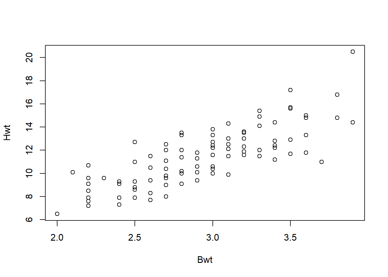
Figure 5.9: Relationship between cats’ body and heart weights.
##
## Call:
## lm(formula = Hwt ~ Bwt, data = catsM)
##
## Residuals:
##     Min      1Q  Median      3Q     Max
## -3.7728 -1.0478 -0.2976  0.9835  4.8646
##
## Coefficients:
##             Estimate Std. Error t value Pr(>|t|)
## (Intercept)  -1.1841     0.9983  -1.186    0.239
## Bwt           4.3127     0.3399  12.688   <2e-16 ***
## ---
## Signif. codes:  0 '***' 0.001 '**' 0.01 '*' 0.05 '.' 0.1 ' ' 1
##
## Residual standard error: 1.557 on 95 degrees of freedom
## Multiple R-squared:  0.6289, Adjusted R-squared:  0.625
## F-statistic: 161 on 1 and 95 DF, p-value: < 2.2e-16## (Intercept) Bwt
## -1.184088 4.312679We would like to assess the variability of our model and its coefficients.
If we had a different sample from the same population, how much would our estimated line move? What about confidence intervals for the intercept and slope? This is where the bootstrap procedure comes in.
# How can we make a confidence interval for these parameters? Use the bootstrap
# This function returns the coefficients of a regression model fitted to a bootstrap sample.
# The ind parameter gives the indices of the bootstrap sample; orig_data[ind,] is the bootstrap sample values.
estimator <- function(orig_data, ind) {
  model_b <- lm(Hwt ~ Bwt, orig_data[ind, ])
  coef(model_b)
}

# Create 1000 bootstrap replicates of the coefficients for the cat data
boot_repl <- boot::boot(catsM, estimator, 1000)
boot_repl
##
## ORDINARY NONPARAMETRIC BOOTSTRAP
##
##
## Call:
## boot::boot(data = catsM, statistic = estimator, R = 1000)
##
##
## Bootstrap Statistics :
## original bias std. error
## t1* -1.184088 -0.023249544 1.1351073
## t2* 4.312679 0.006340115 0.4006028# Compute a 95% confidence interval, based on the bootstrap replicates
# index=1 is the first statistic, this is a ci for the intercept of the regression model
boot::boot.ci(boot_repl, type = "bca", index = 1)## BOOTSTRAP CONFIDENCE INTERVAL CALCULATIONS
## Based on 1000 bootstrap replicates
##
## CALL :
## boot::boot.ci(boot.out = boot_repl, type = "bca", index = 1)
##
## Intervals :
## Level BCa
## 95% (-3.425, 0.924 )
## Calculations and Intervals on Original Scale# index=2 is the second statistic, this is a ci for the slope of the regression model
boot::boot.ci(boot_repl, type = "bca", index = 2)## BOOTSTRAP CONFIDENCE INTERVAL CALCULATIONS
## Based on 1000 bootstrap replicates
##
## CALL :
## boot::boot.ci(boot.out = boot_repl, type = "bca", index = 2)
##
## Intervals :
## Level BCa
## 95% ( 3.590, 5.119 )
## Calculations and Intervals on Original Scale# The pairs of intercept and slope are in the `t` value of the list `boot_repl`
# We can plot each line from each bootstrap sample to get an idea of how our estimate could have varied
boot_repl$t[1:5, ]## [,1] [,2]
## [1,] -2.437597 4.807250
## [2,] -1.327428 4.340109
## [3,] -0.701412 4.090691
## [4,] -1.631726 4.473434
## [5,] -1.544259 4.477614plot(catsM[, 2:3])
abline(a = coef(model)[1], b = coef(model)[2], col = 2, lwd = 3)
tmp <- mapply(abline, boot_repl$t[, 1], boot_repl$t[, 2], MoreArgs = list(col = scales::alpha(rgb(0, 0, 0), 0.05)))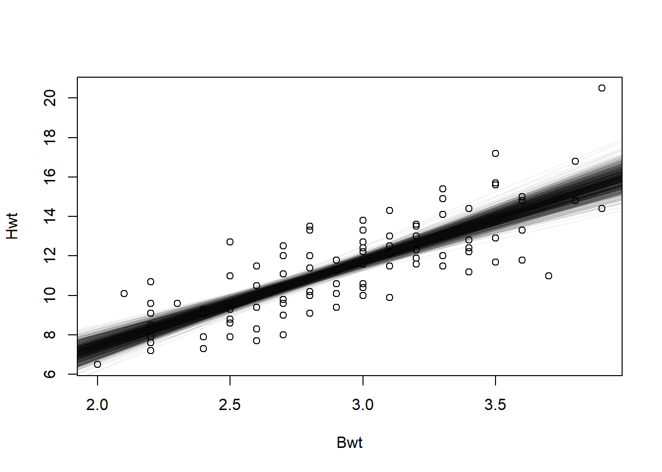
Figure 5.10: Estimated lines created through bootstrap.
5.5 Random Forests
Random forests can be used to build predictive models for a response variable based on a set of predictors. The predictors and response can be of any type. The model does not have interpretable parameters like a slope and intercept, but the regression function or prediction function is not restricted to being a line.
Put simply, if the goal is prediction, the random forest is a good option. How random forests work is somewhat complicated, so we will omit the details. The additional resources section contains some educational material on random forests.
To apply random forest, we assume that the observations are independent and there are no outliers in the data.
5.5.1 Examples Using R
To show how random forests differ from regression, we will simulate a set of data.
## Warning: package 'randomForest' was built under R version 4.3.3## randomForest 4.7-1.1## Type rfNews() to see new features/changes/bug fixes.##
## Attaching package: 'randomForest'## The following object is masked from 'package:ggplot2':
##
## marginset.seed(440)
# invent nonlinear data
x <- rnorm(500)
y <- 2 * sin(x * 4) + rnorm(100, sd = .8)
trim <- x < -2
trim2 <- x > 2
trim <- as.logical(trim + trim2)
# plot data
example_data <- cbind(x[!trim], y[!trim])
plot(example_data, ylab = "y", xlab = "x")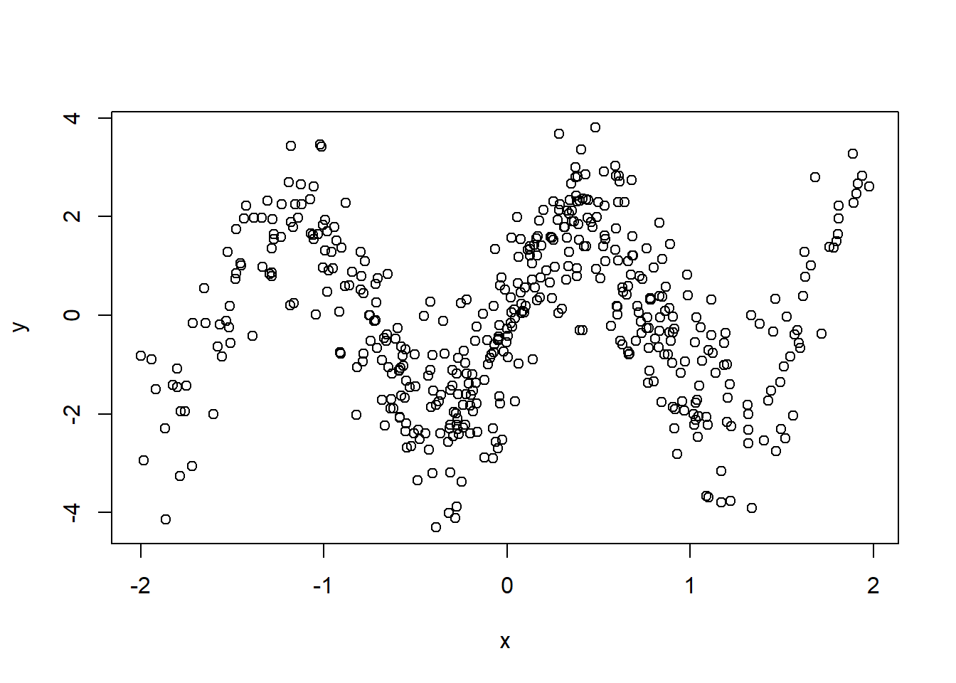
Figure 5.11: Scatterplot of simulated data showing no linear relationship.
Notice how this data clearly does not have a linear relationship. We will explain how to build a random forest for this data.
The caret package will be used to build random forest predictive models. This package includes many different types of predictive models. To train a random forest model, we set the method argument to "rf". This function is based on code from the randomForest package.
Random forests have a number of parameters, we will cover the two most important ones:
- the number of trees in the forest,
ntree, and - each leaf on the tree contains two nodes, chosen from a set of size
mtry.
Building a random forest involves training or building a bunch of random forests with different parameters and choosing the forest with the highest predictive capacity metric.
The predictive capacity metric depends on whether or not your outcome is continuous or categorical. For continuous predictions, the metric is mean squared error, just like in regression.
# the predictors must be a matrix subjxcolumn
x <- matrix(x, ncol = 1)
colnames(x) <- "x"

# train the model
# ntree is the number of trees
# mtry=is a tuning parameter limited by the number of predictors, we only have 1 predictor here.
grid_par <- expand.grid(mtry = 1)
model <- caret::train(x = x, y = y, method = "rf", tuneGrid = grid_par, ntree = 100)
## Warning: package 'caret' was built under R version 4.3.3## Loading required package: lattice## Warning: package 'lattice' was built under R version 4.3.3##
## Attaching package: 'lattice'## The following object is masked from 'package:faraway':
##
## melanoma##
## Attaching package: 'caret'## The following object is masked from 'package:survival':
##
## cluster## Random Forest
##
## 500 samples
## 1 predictor
##
## No pre-processing
## Resampling: Bootstrapped (25 reps)
## Summary of sample sizes: 500, 500, 500, 500, 500, 500, ...
## Resampling results:
##
## RMSE Rsquared MAE
## 1.14985 0.5617973 0.9109683
##
## Tuning parameter 'mtry' was held constant at a value of 1# we want to predict values between -2 and 2
nd <- matrix(seq(-2, 2, l = 100), ncol = 1)
colnames(nd) <- "x"
# generate predictions
preds <- predict(model, newdata = nd)
# plot results
plot(example_data)
lines(c(nd), preds, col = 2)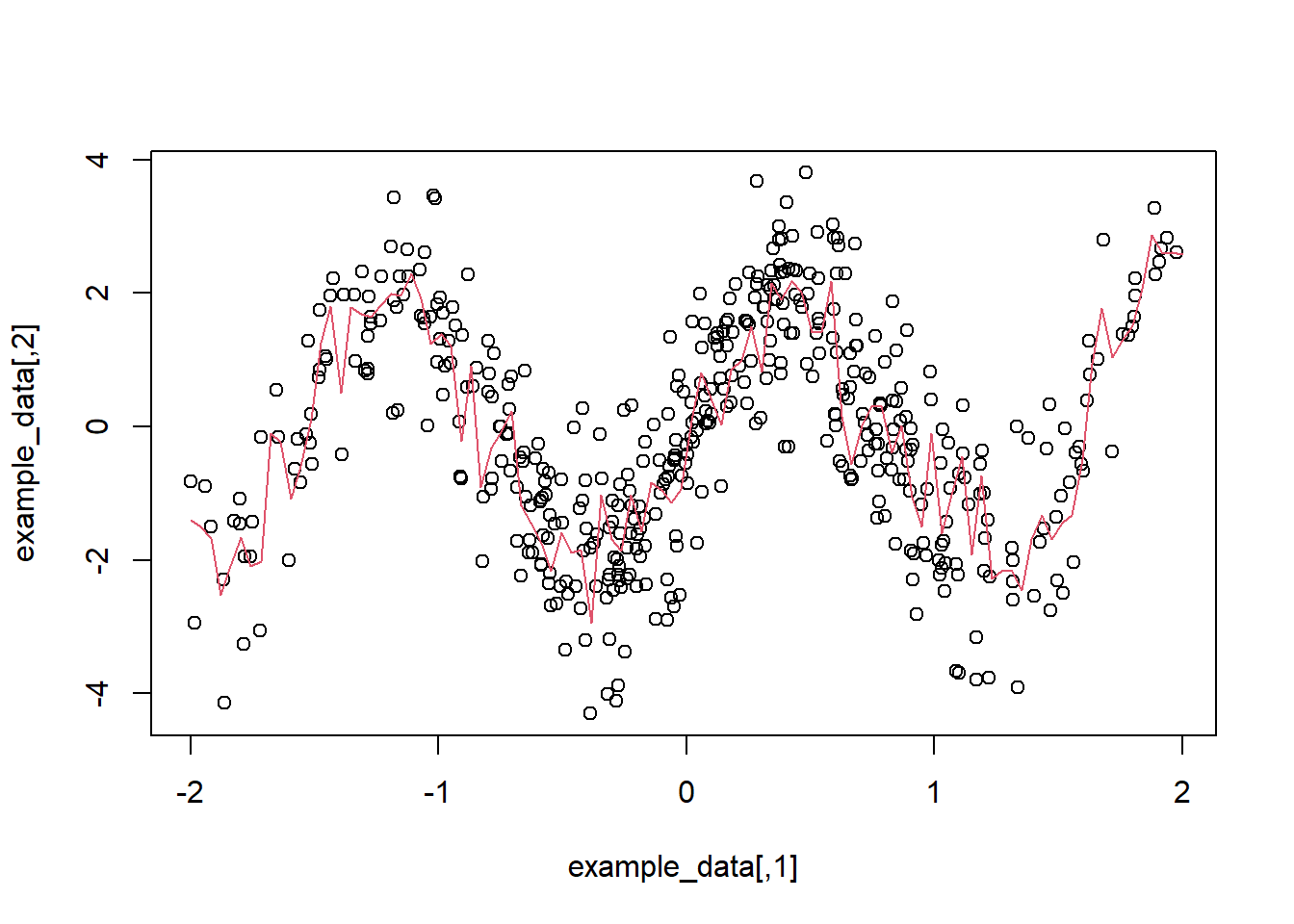
Figure 5.12: The red line shows the prediction obtained through random forest.
The caret package will be used to build random forest predictive models. This package includes many different types of predictive models. To train a random forest model, we set the method argument to "rf". This function is based on code from the randomForest package.
Random forests have a number of parameters, we will cover the two most important ones:
Notice how non-linear the prediction function is? We also have a root mean square error of 1.16, R-squared of 0.5, and mean absolute error of 0.9. These three values are useful for prediction purposes.
The random forests can also be used to predict categorical variables. We will demonstrate how this can be done by building a model that predicts the species of the iris plants based on the four predictors in the data set. For categorical data, there are two metrics output by the train() function.
- accuracy: the proportion of time the right category is selected; and
- \(\kappa\) value: the proportion of time the right category is selected normalized by the probability of selecting the right category by chance. This metric takes into account that correct category selection may happen by chance.
# iris data
grid_par <- expand.grid(mtry = 1:4)
model <- caret::train(x = iris[, 1:4], y = iris$Species, method = "rf", tuneGrid = grid_par)
model
## Random Forest
##
## 150 samples
## 4 predictor
## 3 classes: 'setosa', 'versicolor', 'virginica'
##
## No pre-processing
## Resampling: Bootstrapped (25 reps)
## Summary of sample sizes: 150, 150, 150, 150, 150, 150, ...
## Resampling results across tuning parameters:
##
## mtry Accuracy Kappa
## 1 0.9392946 0.9077114
## 2 0.9426003 0.9125928
## 3 0.9450316 0.9162926
## 4 0.9444510 0.9153989
##
## Accuracy was used to select the optimal model using the
## largest value.
## The final value used for the model was mtry = 3.## [1] setosa setosa setosa setosa setosa setosa
## Levels: setosa versicolor virginica# probability of being in each group based on model
predict(model, newdata = head(iris[, 1:4]), type = "prob")## setosa versicolor virginica
## 1 1 0 0
## 2 1 0 0
## 3 1 0 0
## 4 1 0 0
## 5 1 0 0
## 6 1 0 0We can have a large number of predictors. Let’s look at the cars data. We wish to predict the car’s price from a large number of predictors.
##      Price Mileage Cylinder Doors Cruise Sound Leather Buick
## 1 22661.05   20105        6     4      1     0       0     1
## 2 21725.01   13457        6     2      1     1       0     0
## 3 29142.71   31655        4     2      1     1       1     0
## 4 30731.94   22479        4     2      1     0       0     0
## 5 33358.77   17590        4     2      1     1       1     0
## 6 30315.17   23635        4     2      1     0       0     0
##   Cadillac Chevy Pontiac Saab Saturn convertible coupe hatchback
## 1        0     0       0    0      0           0     0         0
## 2        0     1       0    0      0           0     1         0
## 3        0     0       0    1      0           1     0         0
## 4        0     0       0    1      0           1     0         0
## 5        0     0       0    1      0           1     0         0
## 6        0     0       0    1      0           1     0         0
##   sedan wagon
## 1     1     0
## 2     0     0
## 3     0     0
## 4     0     0
## 5     0     0
## 6 0 0## [1] 17# we will tune mtry between 1 and 9 , but it can go to 18
grid_par <- expand.grid(mtry = 1:9)
model <- caret::train(x = cars[, -1], y = cars$Price, method = "rf", tuneGrid = grid_par)
model## Random Forest
##
## 804 samples
## 17 predictor
##
## No pre-processing
## Resampling: Bootstrapped (25 reps)
## Summary of sample sizes: 804, 804, 804, 804, 804, 804, ...
## Resampling results across tuning parameters:
##
## mtry RMSE Rsquared MAE
## 1 5949.350 0.8752130 4517.518
## 2 3624.750 0.9082719 2680.873
## 3 2829.858 0.9286917 2074.238
## 4 2494.819 0.9398563 1797.216
## 5 2326.131 0.9458389 1650.106
## 6 2252.660 0.9481963 1581.958
## 7 2218.040 0.9492911 1548.127
## 8 2206.271 0.9496153 1536.879
## 9 2209.485 0.9493266 1534.859
##
## RMSE was used to select the optimal model using the smallest value.
## The final value used for the model was mtry = 8.## 1 2 3 4 5 6
## 20714.63 21575.53 30943.25 32073.94 33889.83 31979.89## [1] 22661.05 21725.01 29142.71 30731.94 33358.77 30315.17